Investigating Emergence
On understanding practical and other applications of emergent systems.
- Abstract
- Ant Colony Optimisation
- Final Product
- Explanation
- Brute Force
- ACO
- Generating Routes
- Calculating Distances
- Laying Pheromones
- Optimisation
- Finding Intersections
- Orientation
- Development
- Prototype
- Modifications
- Conclusion
- Information
- Ant Colony Simulation
- Boids
- Final Product
- Explanation
- Limits
- Separation
- Cohesion
- Alignment
- Development
- Prototype
- Modifications
- Conclusion
- Information
- Reaction Diffusion
- Final Product
- Explanation
- Initialisation
- Diffusion
- Simulation
- Development
- Prototype
- Conclusion
- Information
- Machine Learning
- Final Product
- Explanation
- main.jl
- train.jl
- initialise.jl
- forward_propagation.jl
- cost.jl
- backpropagation.jl
- Final steps
- Development
- Prototype
- Modifications
- Conclusion
- Information
- Conclusion
- Glossary
- Literature Review
- Emergence in general
- Ant Colony Optimisation
- Ant Colonies
- Boids
- Reaction Diffusion
- Machine Learning
- Appendix A
- Appendix B
- Appendix C
- Appendix D
- Bibliography
Abstract
Emergence is a property that we see all the time in systems with simple rules - chaos. More precisely, unpredictability. Emergent behaviour is when something unexpectedly complex appears from an application of its rules. We see this all the time in the natural world: ant colonies, birds flocking, and even life itself are all bizarre consequences of rules that we can fully understand. I set out to understand the practical applications of emergence in solving problems we face, as well as its ability to model natural systems that were previously hard to understand.
Quite a few mathematical problems are particularly hard to solve more efficiently than simply testing every possible answer, and a problem arises when using brute force to find the solution simply takes too long. A simple example is the travelling salesman problem: a merchant wants to travel in a loop through a series of cities (reaching each only once). What's the shortest distance they must travel? There is a correct answer, but no one has found a way of finding it without testing every path. This is where emergence comes in - by using simple systems, often modelled after nature, we can generate a very good solution in a tiny fraction of the time it would otherwise take. However, the solution we find isn't guaranteed to be the best solution, it is a heuristic [1], but finding approximate solutions to problems like this is crucial all the time. This same process is, for example, what drives machine learning, which is a crucial part of our modern world.
I've made 5 different emergent models. In this report, I will look at each one in turn, first showing the product, then how they work, and then my own conclusions about what it shows us about emergence. Firstly, I look at Ant Colony Optimisation, which shows a clear practical application of emergence. Secondly, I model an Ant Colony, which demonstrates emergence's ability to model complex behaviour from the natural world. Thirdly, I simulate boids, which show how another natural system can be explained with emergence. Fourthly, I made a reaction-diffusion model which shows a different style of emergent behaviour to the others. Finally, I made a machine learning model, which again demonstrates emergence's power and applications in the real world. I tried to pick models which cover a broad range of emergent behaviours and address both aspects of my title. I wrote all the code for all the models apart from some parts of the machine learning model.
In my EPQ, I aim to investigate a number of different emergent systems - primarily by modelling them myself. Some of the results are beautiful, others are underwhelming, but they all offer some insight into problem solving or nature itself. Some aspects of nature, for example bird flocking, were unexplained phenomenon, but emergent systems provide an explanation. Life itself is an emergent property; cells are simple, yet people are smart. How does that happen? Society from people, wetness from water molecules, buildings from concrete, ant colonies from ants, these are all emergent systems. I do not have scope in this project to examine why consciousness emerges from cells (or similarly large questions), but emergence does seem to be a fundamental property of the universe and in my EPQ I set out to learn more about it.
Ant Colony Optimisation
Ant colonies have inspired an excellent heuristic for the travelling salesperson problem (TSP) (Eddie Woo, 2015). No one has found a practical algorithm to solve this or other similar NP-hard problems but there are several reliable heuristics.
Final Product
In TSP, the times to solve the problem by brute force (the best-known algorithmic solution) get exponentially larger.

1: 10 Points took 1 second.

2: 13 points took 23 mins 10 seconds.
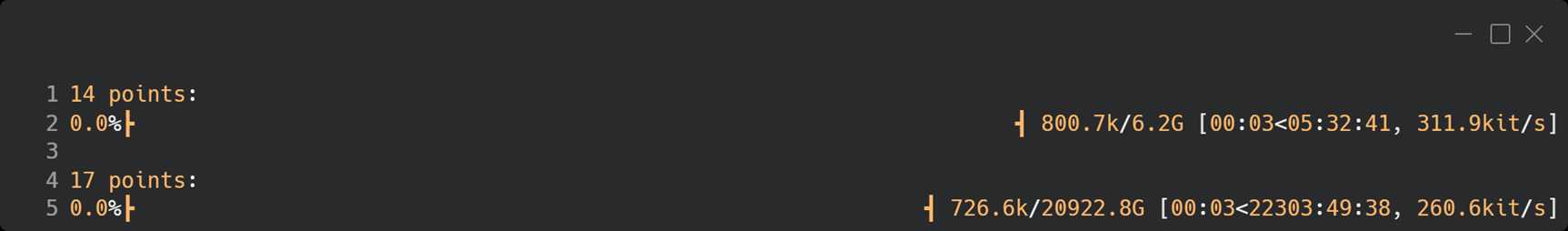
3: 14 & 17 points projected to take 5:32:44 and 22303:49:41 respectively.
As you can see, the estimated time to solve/the actual time required (shown on the right) goes from merely a second for 10 points, to 23 minutes for 13, then 5.5 hours at 14 points and over 2.5 years for 17 points. The point of a good heuristic for TSP is to provide a guess at a solution while making huge savings on time invested.
An Ant Colony Optimisation (ACO) approach to TSP follows a loop:
- Release ants to go between points, they are biased to follow pheromone trails.
- Score how far the ants walked and use that to determine the intensity of pheromones to place along that route.
- Optionally, some simple further optimisation can be performed on the route the ants walked.
- Remove some fraction of the pheromones so the numbers remain useful.
Applying these steps can produce the following (note the times taken):
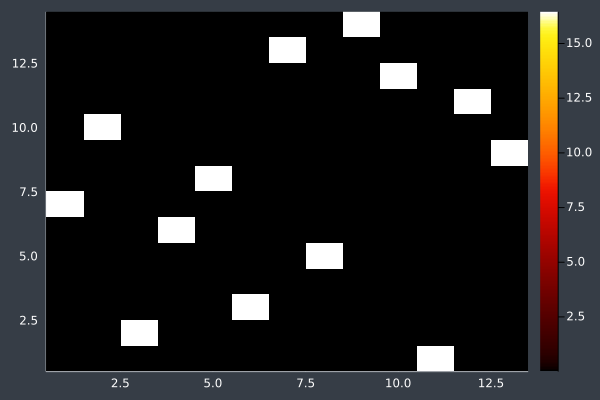
ACO usually reached the correct solution, or a solution that was almost identical to the brute force solution, at 10 points (and lower):
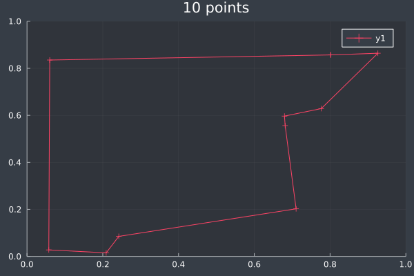
4: 10 points in 0 seconds with ACO (no further optimisation) (2000 iterations, 20 ants).

5: Same 10 points in 1 second by Brute Force.
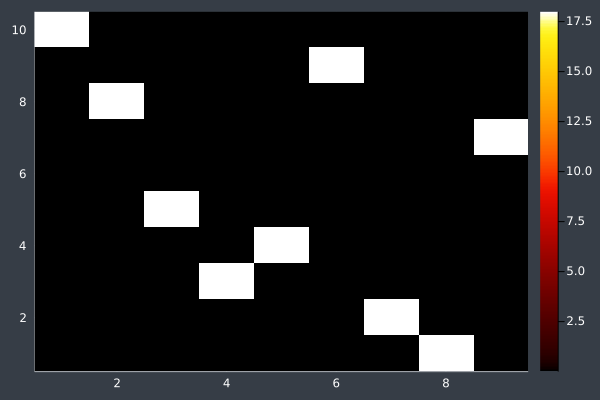
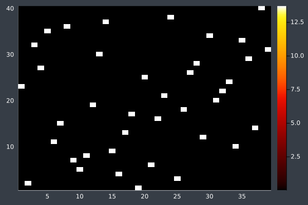
6: Pheromone intensity graphed. Y-axis shows the current point, and the X-axis shows the point to move to. The fewer bright points there are, the more certain ACO is of its solution.
At 14 points we can see that ACO usually reaches a solution it is confident in, but not always (shown in the lower example, where we can make improvements ourselves). With some optimisation the approximation is still good:
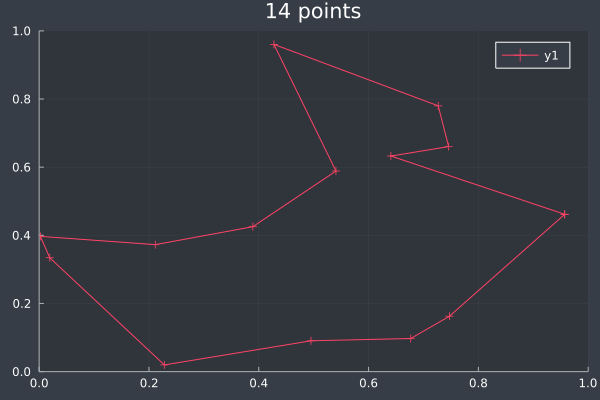
7: 14 Points in 1 second with ACO (optimisation) (2000 iterations, 20 ants, small optimisations each iteration).
8: Pheromone intensity.
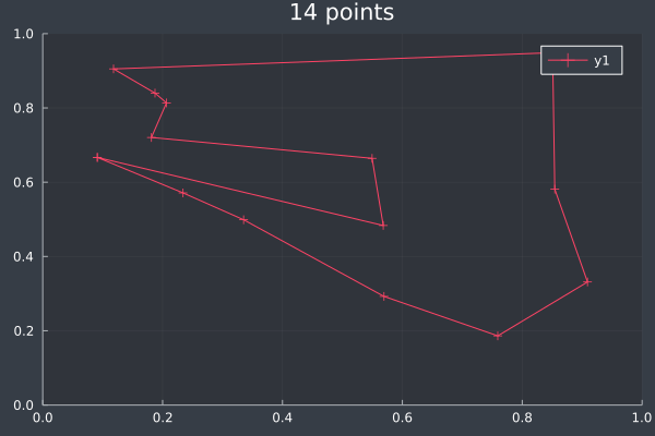
9: 14 Points in 1 second with ACO (optimisation) (2000 iterations, 20 ants, small optimisations each iteration).
10: Pheromone Intensity.
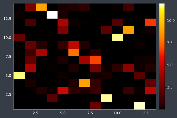
Without subtle optimisation (max. 10 changes) each iteration, the ants do not always have enough time to reach a solution after only 2000 iterations:
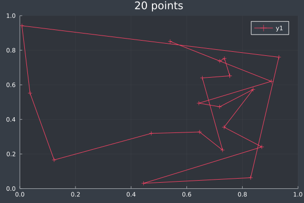
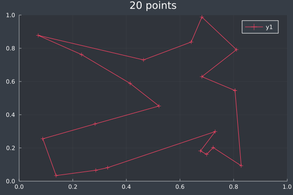
11: 20 Points in 1 second with ACO (no optimisation at any stage) (2000 iterations, 20 ants).
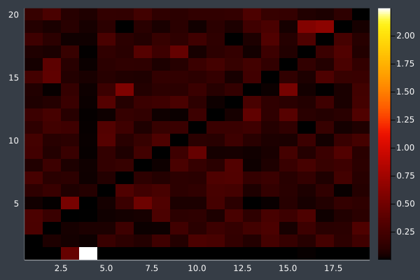
12: We can see the uncertainty in the heatmap.
13: 20 Points in 2 seconds with ACO (optimised) (2,000 iterations, 20 ants).
Sometimes the algorithm would slip up with 2,000 iterations at 20 points. So I gave the ants 20,000 iterations (~13 seconds) and have not seen an absurd solution in my tests. This was very exciting and I wanted to push the algorithm further. In the cases where I could see improvements that could be made to the solutions, it was interesting to see that after 20k iterations the ants had still converged on one route. This demonstrates the nature of ACO as a heuristic and not an algorithm: the ants may give you an answer with utter certainty, but that does not mean that they are right.
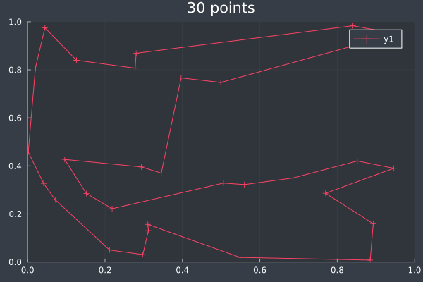
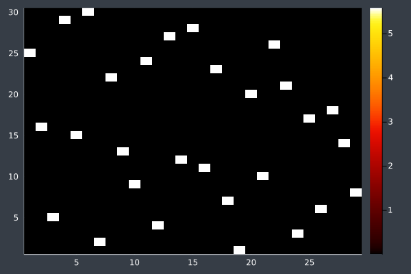
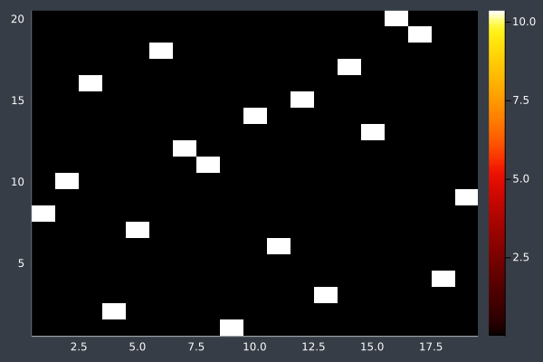
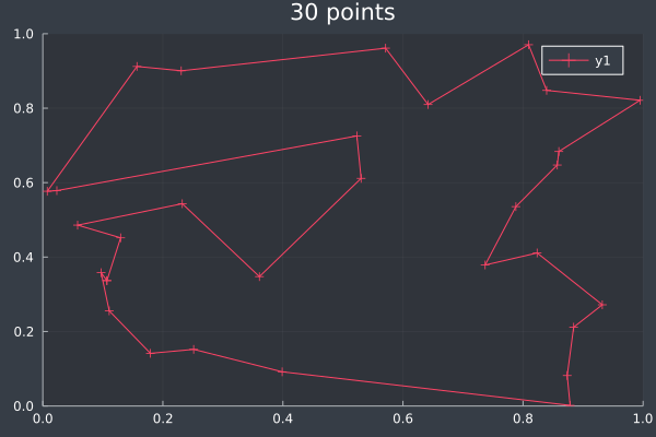
14: 30 Points, 20k iterations, 20 ants, optimised, in 29 seconds. Initial pheromone intensity 1.0.
I raised the number of ants to 50 and the starting pheromone intensity to 10.0. With the larger number of points this should give the ants more opportunity to find potential routes without accidentally ruling them out due to evaporation.
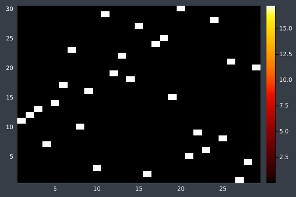
15: 30 Points, 50 ants, starting intensity 10.0.
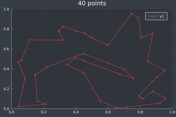
16: 40 Points, otherwise same, in 2 mins 29 secs.
With these conditions, ACO hit its limit of providing good solutions at 50 points. I do not doubt that, by increasing the number of ants and iterations, ACO could solve even larger problems. However, I decided to stop pushing here. As you can see, without changing the conditions, ACO is producing obviously bad solutions. However, we also saw this earlier before we increased the number of ants and steps and so I expect that ACO would work for any number of points if given sufficient time and ants.
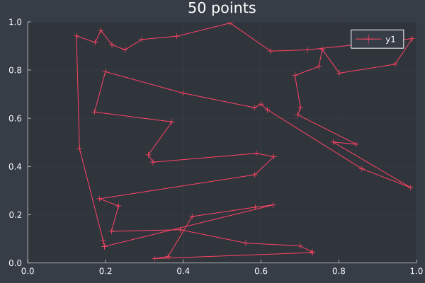
17: 50 Points in 3 mins 54 seconds (without final optimisation pass).
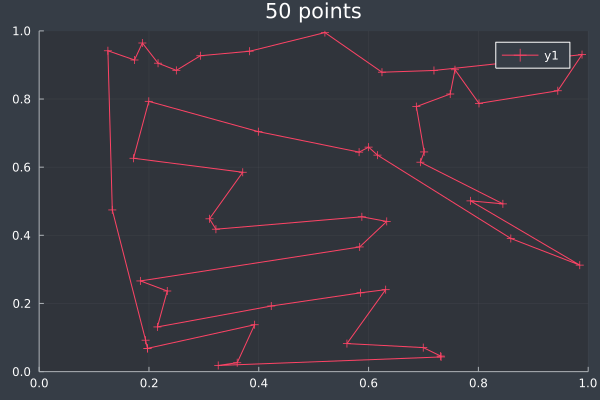
18: With final pass.
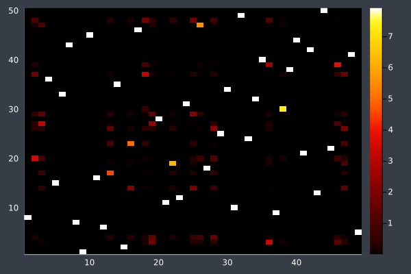
19: Pheromone intensities.
Explanation
The program can be split into 3 different sections: Brute force, ACO and optimisation. Brute force and ACO are independent but the optimisation requires some initial route to improve upon. I've separated it out from the ACO section to make it clear that it is not necessary for ACO and that it moves slightly further from biomimicry to produce a more reliable solution faster.
Brute Force
A brute force algorithm is simple: test every possible combination of points and save the best one. We know that this will find the correct solution because we know it is testing every possible order.
"""
brute(points::Vector{Vector{Float64}}) -> (order = Vector{Int}, best_score = Float64)
    Uses brute force to find the shortest route through `points`, returning to the starting point.

Since it does not matter where we start, the first and last points are both 1.
"""
function brute(points::Vector{Vector{Float64}})
    # A variable which will store the distance of
    # the shortest route the algorithm has found.
    Best_score = Inf

    # A Vector which will store the best route.
    Best = Int[]

    # For each possible order...
    # (assuming the order starts and ends at 1)
    for order in ProgressBar(permutations(2:length(points), length(points) - 1))

        # Calculate the distance of the order
        distance = route_s(points, order)

        # If the distance is shorter than the current best...
        if distance < best_score

            # Save the new distance and best order
            best_score = distance
            best = deepcopy(order)

        end # if
    end # for

    # Add the first and last point 1 (which was assumed)
    prepend!(best, 1)
    append!(best, 1)

    return (order = best, distance = best_score)
end # function
ACO
Each iteration of ACO for TSP begins by generating a number of routes through the points equal to the number of theoretical ants being released. At each decision in the routes, where the ant goes is biased only by the current pheromone intensity pointing in that direction. Otherwise the decision is random. Then the program scores each route by its distance and adds pheromones to the trail in the following relationship:
$$Ph_{route}=\left(\frac 1 S \right)^G$$
Where $G$ is the greed [2] of the system and $S$ is the total distance of the route.
Then there is some amount of evaporation. The Pheromone intensity at each point is reduced by a factor $E$. Since the fraction of pheromone being taken away is constant everywhere, this ensures that the pheromone intensity can never increase above a certain limit and it reduces the intensity through routes that are never used.
This cycle repeats for the specified number of iterations.
"""
    ants(points, [iters, n, evaporation, greed, optimise]) -> (order, distance, ph)

Biomimicry with ant colonisation!
Returns a route by sending `n` ants around in a loop.
"""
function ants(points::Vector{Vector{Float64}}, iters = 500, n = 20, evaporation = 0.1, greed = 2.0, optimise = true)

    # Create a matrix which will store the pheromone intensities.
    Ph = fill(10.0/length(points), length(points), length(points) - 1)

    # Begin iterating...
    for _ in ProgressBar(1:iters)

        # Generate n routes through the points using the pheromone values.
        Orders = route(points, ph, n)

        # If each route should be optimised slightly...
        if optimise

            # For each of the suggested orders...
            for order in orders

                # Run optimisation (decrosses most crossed lines)
                # on each order, limited to making 3 changes.
                Order = decross(order, points, 3)

            end # for

        end # if

        # Calculate the distances of each route.
        Distances = route_s(points, orders)

        # Place pheronmones on each route using the distances.
        Ph += lay_ph(orders, distances, points, greed)

        # Allow some fraction of the pheromones to evaporate
        # The fraction is constant in all places.
        Ph = (1-evaporation) .* ph

    end # for

    # Save the final pheronomes
    ph_out = deepcopy(ph)

    #== Find the preferred route ==#

    # An array to store the preferred route.
    Best = Int[0 for _ in 2:length(points)]

    # A variable to store the current location of the
    # ant which follows the preferred route.
    Current = 1

    # For each stop the ant must make...
    for I in 1:length(points)-1

        # Set the pheromones intensities of points
        # the ant has already visited to -Infinity.
        ph[current, :] = [x+1 in best ? -Inf : ph[current, x]
                            for x in 1:length(ph[current, :])]

        # Find the point with the highest pheromone intensity.
        p = findmax(ph[current, :])[2] + 1

        # Save this point.
        best[i] = p

        # Move the ant to the new point.
        current = p

    end # for

    # Add 1s to the beginning and end of route (assumed).
    prepend!(best, 1)
    append!(best, 1)

    return (order = best, distance = route_s(points, best[2:end-1]), ph = ph_out)

end # function
Generating Routes
In order to send virtual ants around through the points, we need to generate routes. This function generates one route for each of the ants. I use weighted sampling to pick a point.
"""
route(points, ph, n) -> Vector{Vector{Int64}}

Generate `n` routes through `points` where the pheromone intensities are `ph`.
Uses weighted random sampling.
"""
function route(points::Vector{Vector{Float64}}, ph::Matrix{Float64}, n::Int)

    # Create a heromone which will hold the routes
    orders = Vector{Int64}[]

    # For each route that needs to be createI.
    for _ in 1:n

        #== Get a route ==#

        # Create a variable which will temporarily store the route.
        order = Int[0 for _ in 2:length(points)]

        # Store the point where the ant currently is.
        current = 1

        # For each point the ant needs to travel thrIh...
        for i in 1:length(points)-1

            # Store possible points the ant can go to
            # which is the list of points excluding the ones already visited.
            _Ps = [x for x in 2:length(points) if !(x in order)]

            # Store the Pheromone values at those point from the current point.
            _Phs = [ph[current, x-1] for x in 2:length(points) if !(x in order)]

            # Pick the next point randomly (weighted  heromoneeronome trails).
            p = sample(_Ps, pweights(_Phs), 1)[1]

            # Save that new point.
            order[i] = p

            # Move the ant to the new point.
            current = p

        end # for

        # Store the route in the list of routes.
        push!(orders, order)

    end # for

    return orders

end # function
Calculating Distances
The simulation calculates the distance of each route on request. It would be absurd to calculate the distance of each route ahead of performing ACO since calculating each distance solves TSP anyway. However, I could have calculated a table of distances between points ahead of releasing the ants. As you've seen in the examples, ACO ran fast enough that this was not a significant issue so I chose not to make this improvement. In a larger scale implementation that was required to run faster this should be implemented.
"""
    route_s(points, order) -> Float64

Returns the distance of the route `order` through `points`
(in n-dimens“””s).
"""
function route_s(points::Vector{Vector{Float64}}, order::Vector{Int})

    # Create a variable to store the distance.
    distance = 0.0

    # For each point in the route (plus an endIint)...
    for i in 1:length(order)+1

        #==
        Add the distance between the previous point
        (assumed starts at 1) and then next point to
        the distance variable.
        ==#
        distance += s(points[get(order, i-1, 1)], points[gIt(order, i, 1)])

    end # for

    return distance

end # function
Laying Pheromones
The pheromones are laid as described below. The $\frac 1 S$ aspect is intuitive enough - shorter overall route lengths should increase pheromone intensity. However, I discovered the use of a greed parameter $G$ through looking at other implementations of ACO and I found, through their approaches and my own experimentation, that a good greed was 2. The greed changes the amount which the program is drawn towards routes it found with a low distance. The real life scenario this model is based off would have a greed of 1. The amount of pheromones along a route with real ants is equal to the number of ants which could follow along the route in a given time. If the route is shorter, the ants can use it more times, so the pheromones will be more intense.
$$f=\frac v {\lambda}$$
Where $f$ is frequency, $v$ is speed, and $\lambda$ is the distance.[3]
"""
    lay_ph(orders, distances, points, greed) -> Matrix{Float64}

Returns a matrix like ph which shows the new pheromones laid down orders.
"""
function lay_ph(orders::Vector{Vector{Int}}, distances::Vector{Float64}, points::Vector{Vector{Float64}}, greed::Float64)

    # Create an empty matrix where the new pheromones can be stored.
    empty = fill(0.0, length(points), length(points) - 1)

    # ForIch order...
    for j in 1:length(orders)

        #== Update the pheromones ==#

        # Create a variable to store the previous point.
        prev = 1

        # For each point in the route...
        for i in orders[j]

            # Add pheromones to the path between the
            # previous point and the next point.
            empty[prev, i-1] += (1/distances[j]) ^greed

            # Save the current point as the previous point.
            prev = i

        end # for

    end # for

    return empty

end
Optimisation
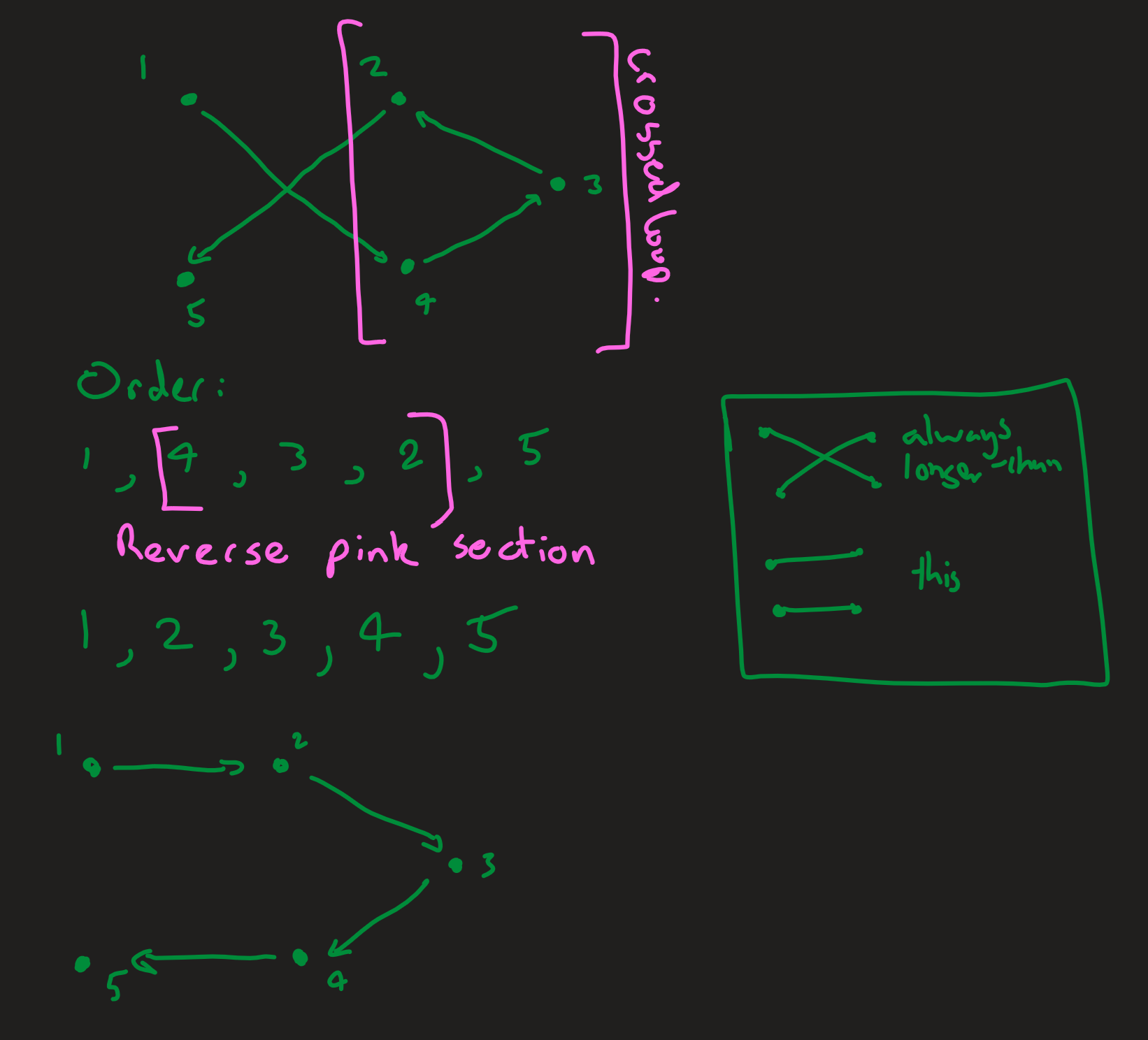
The job of my separate optimisation algorithm is to improve the efficiency of ACO by stopping the ants from following absurd routes with easy optimisations. The simple optimisation I applied was to uncross crossed lines, which would always reduce the length of the route.
Reversing the order of points in the loop of a cross always uncrosses the lines and always reduces the length of the route.
"""
    decross(order, points, [limit]) -> order::Vector{Int}

Return an order were `limit` many changes were
made to remove cross lines from the `order` “””ough
`points`.
"""
function decross(order, points, limit = 100)

    # Create a variable we can test later to see
    # if the algorithm made a change.
    success = false

    #==
    This function is recursive but it needs to
    know to stop at some limit. This also allows
    us to stop the algorithm making too many changes.
    ==#
    if limit > 0

        # Iterate through all the individual paths between points
        # in each rIute.
        for i in 0:length(order)
            for j in i+2:length(order)

                    # Avoid a special case where the algorithm makes
                    # the same change forever.
                    if !(i == 0 && j == length(order))

                        # Find the relevant 4 points.
                        # The first line is p1q1.
                        p1 = points[get(order, i, 1)]
                        q1 = points[get(order, i+1, 1)]

                        # The second line is p2q2.
                        p2 = points[get(order, j, 1)]
                        q2 = points[get(order, j+1, 1)]

                        # If the I lines intersect...
                        if ifintersect(p1, q1, p2, q2)

                            # Remove the cross by reflecting the order
                            # of points in the loop of the intersection.
                            order[i+1:j] = reverse(order[i+1:j])

                            # Track that there was a success.
                            success = true

                            # break out of the loop.
                            break

                        end # if

                    end # if

            end # for
            if success
                break
            end # if
        end # for

    end # if

    # If one pair Ilines was uncrossed...
    if success

        #==
        Run the algorithm again on the new order.
        Since news crosses may have been introduced by
        the uncrossing.
        ==#
        return decross(order, points, Iit-1)

    # Otherwise...
    else

        # End the recursion and return the final order.
        return order

    end # if

end # function
Finding Intersections
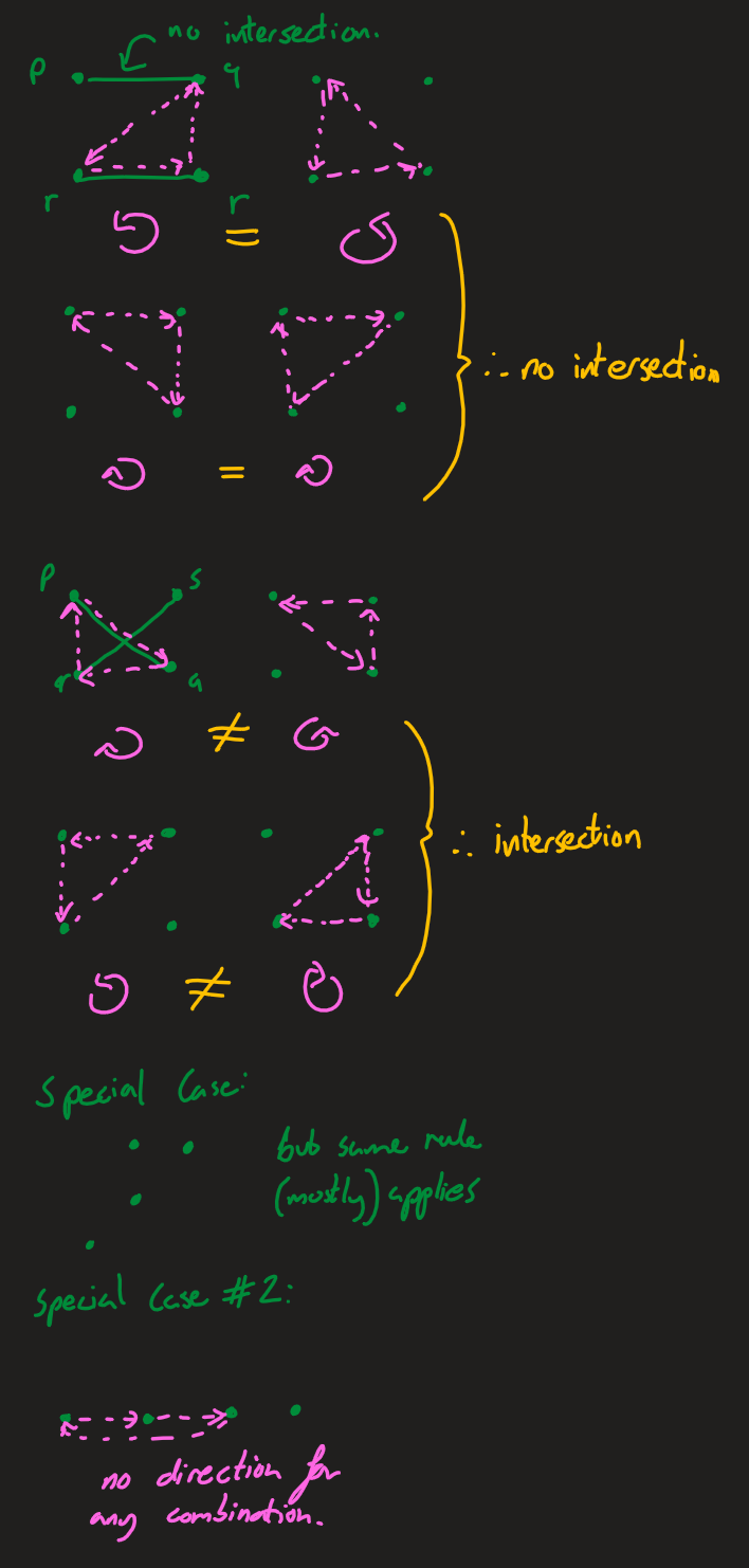
A set of 3 points can be described as clockwise or anticlockwise as defined below. In the most general case, the lines p1q1 and p2q2 intersect if the orientations of p1,q1,p2 and p1,q1,q2 are different and the orientations of p2,q2,p1 and p2,q2,q1 are different ('How to check if two given line segments intersect?', 2013).
There are special cases where three of the points are colinear (lie on the same line). If p,r,q is colinear (and the lines are pq, rs), r may lie on pq or it may simply lie on the sam"""ine and not intersect.
"""
    ifintersect(p1, q1, p2, q2) -> bool

Checks if p1q1 and p2q2 intersect.
"""
function ifintersect(p1, q1, p2, q2)

    # Find the 4 relevant orientations
    o1 = orientation(p1, q1, p2)
    o2 = orientation(p1, q1, q2)
    o3 = orientation(p2, q2, p1)
    o4 = orientation(p2, q2, q1)

    # If the orientations of the two pairs are different
    # then the lines intersect.
    if (o1 != o2) && (o3 != o4)
        return true
    end # if

    # If any of the Special colinear cases...
    if (o1 == 0 && colinearOnSegment(p1, p2, q1)) ||
            (o2 == 0 && colinearOnSegment(p1, q2, q1)) ||
            (o3 == 0 && colinearOnSegment(p2, p1, q2)) ||
            (o4 == 0 && colinearOnSegment(p2, q1, q2))
        return true
    end # if

    # Otherwise the lines do not intersect.
    return false

end # function
Orientation
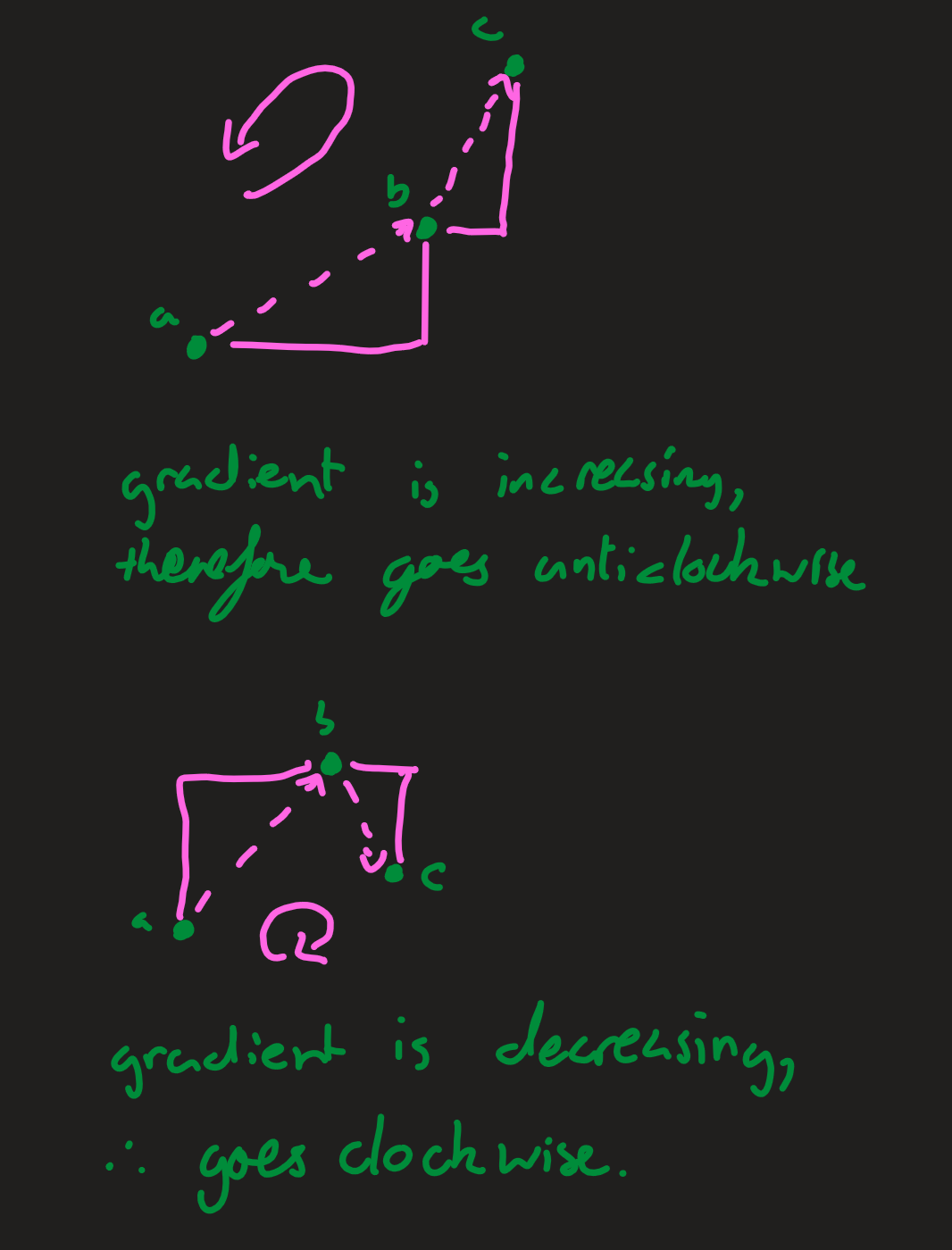
Here we need to calculate if the points are clockwise or anticlockwise. If the gradient between the first two points is less than the gradient between the second two (the third point moves left), then the orientation is anticlockwise. Similarly, if the gradient between the first two points is greater than the gradient between the second two (the third point moves right), then the orientation is clockwise. If the gradients are all the same, then the points are colinear.
For lines pq and rs:
$$m=\frac {dy} {dx} (pq)=q_y-p_y q_x-p_x$$
$$n=\frac {dy} {dx} (qr)=r_y-q_y r_x-q_x$$
If $m>n$, then the points go clockwise, since the second gradient is shallower. If $n>m$, then the points go anticlockwise. The equation which expresses this most easily can be derived as follows:
$$m-n=q_y-p_y q_x-p_x-r_y-q_y r_x-q_x$$
Multiplying by $(p_x-q_x)(p_x-r_x)$ [4]:
$$(q_y-p_y )(r_x-q_x )-(q_x-p_x)(r_y-q_y)$$
This preserves the signs and this function will give a value $>0$ when the points go clockwise, a value of 0 when they are colinear, and a value $< 0$ when they go anticlockwise. The only necessary final step in the code is to lump together all clockwise and anticlockwise cases into having one value [5].
"""
    orientation(p, q, r) -> Int

Returns `1` if the points go clockwise, `-1` if Anticlockwise“””d `0` if they are colinear.
"""
function orientation(p, q, r)

    # This calculation gives a value that is determined
    # by the orientation (direction) o- the points.
    dir = ((-q[2] - p-2]) * (r[1] - q-1])) - ((q[1] - p[1]) * (r[2] - q[2]))

    # If I direction is greater than 0...
    if dir > 0

        # Then the points go clockwise.
        return 1

    # If the direction is less than 0...
    elseif dir < 0

        # Then the points go anticlockwise.
        return -1

    # Otherwise the direction is 0
    else

        # The points are colinear.
        return 0

    end # if

end # function
Special Cases
This case only applies when we already know that the point q lies'on the same line as pr but we don't know if it lies on the same segment, which would tell us if there is a colinear intersection. This case is very rare in randomly generated points but it is worth including.
If q is on the segment, then the following must be true of its coordinates (which, combined, are equivalent to the if statement in the code below):
$$\min(p_x,r_x) \leq q_x \leq \max(p_x,r_x)$$
$$\min(p_y,r_y) \leq q_y \leq \max(p_y,r_y)$$
"""
    colinearOnSegment(p, q, r) -> bool

Given the points are colinear, checks if q lies on pr.
"""
function colinearOnSegment(p, q, r)

    # Knowing that q lies on the same line pr,
    # check if it is betweenIem or not on the segment...
    if q[1] <= max(p[1], r[1]) && q[1] >= min(p[1], r[1]) &&
            q[2] <= max(p[2], r[2]) && q[2] >= min(p[2], r[2])
        return true
    end # if

    return false

end # function
Development
In addition to the code above, I wrote 4 small functions: the first one to generate the points, the second to calculate the distance between two points and the final two to visualise the routes and pheromones after the calculations. These can be found in Appendix A.
Prototype
My first prototype was functional, though some of the methods I was using were attempts to compensate for other mistakes, which I fixed later. Only one ant was sent out each iteration and the trails did not evaporate. There also was no optimisation to avoid crossing lines. I did see some good results (see below), but they were not as consistent and the overall structure was much more clunky. Initially I also used a (negative) exponential function to lay the pheromones, this is because I was worried about the 1/x function being too sharp. At the time I think that this was a valid concern because I only used one ant but it did not reflect the system the program was based off.
Modifications
Throughout development I experimented with a number of different starting pheromone intensities and methods of laying down pheromones. Eventually I would settle into the system above (which was also the simplest). However, before I reached that conclusion, I tried to improve the efficiency of the algorithm by weighting the starting pheromone intensities by the distance between the two points and by multiplying the pheromones to be added to each area by 1/the distance of the path between the two points. In a way, these improved the program, but not in a real way. Both changes moved the program towards a nearest-neighbour approach, which is another much simpler heuristic for TSP. Eventually I realised that laying pheromones and the starting conditions were not what was limiting the quality of my program.
In the next version, I made most of the changes to make the program into its final state. I cleaned up the code and broke it into more convenient functions, which could run for multiple ants and I added the ability to plot the pheromone intensities on a heatmap. I also added the separate optimisation algorithm which went through some iteration to reach a state where it worked as intended. The most interesting part of this was finding the best algorithm to uncross the lines. Initially, I thought to swap the locations of the two end points of the cross in the list. I think that repeating this process would eventually uncross all the lines, but it would require many more steps than the final reflection idea I came to later by drawing out a number of crossed lines with points on paper and figuring out how I intuitively wanted to uncross them and what this would do to the list of points.
Conclusion
Mapping software needs to find routes through points like in TSP (similar problems, without loops, also face the same issues with brute force) all the time so finding a good way to approximate a solution is important to navigation.
I am pleased with how effective the algorithm ended up being at finding a good solution through the points and there is clearly potential in this kind of approach in finding heuristics for other NP-hard problems.
Since it was the last project I undertook for my EPQ, development of ACO went pretty smoothly although there certainly were some hiccups in figuring out how the process should work. If I could work further on ACO, I would work to include reflections (routes going in opposite directions should be considered the same), apply my optimisation more consistently to the routes (currently until the final route it only optimises the first 3 crosses which means that the route around the start/end point is highly optimised but not the rest), and give the ants a better starting set of weights, so that they find a better route faster. In the end, as shown above, none of these issues are deal breakers for ACO.
Making this model, I learnt a lot about emergence's potential to provide heuristic solutions to real-world problems. Many NP-hard problems are of a similar type to the Travelling Salesperson problem and a better algorithm, while not impossible, seems unlikely. I love how simple and effective Ant Colony Optimisation's approach is to this problem. The Wikipedia page for ACO lists countless possible applications for this technique [6] including edge detection, scheduling and nanoelectronics design. This is an amazing breadth of applications for such a simple idea, and working to implement my own version helped me appreciate the power of it.
Information
Language used: Julia
Packages imported: ProgressBars, Plots, Combinatorics, StatsBase
Ant Colony Simulation
Ant Colonies themselves are excellent examples of emergent behaviour. There is no central intelligence directing the ants and yet they are able to: manage numbers of ants performing different roles, coordinate to collect food, and navigate around their environment efficiently. They do this primarily using a couple of mechanisms (because ants are real things, their behaviour is in fact quite complex but it is simplified in every model I have seen): counting other ants to manage jobs, using pheromones to signal food, or that food has run out and using pheromones, an internal pedometer, and landmarks to navigate.
Final Product
In these simulations, each ant's location is represented on the grid below, this limited the capabilities of this model and actually made it harder to create in some ways; I'll get into this more later.
Ant-colony like behaviour can be seen in this model: ants are moving back and forth between sources of food (not shown in simulation 1) and they are doing this by laying down pheromone trails (not shown in simulation 1).

20: Simulation 1
In simulation 2 the ants, pheromone intensities and food sources are shown but not on the same gif. In this simulation, pheromone intensities did not evaporate. This simulation shows a serious problem where the ants get stuck at the bottom of the area.
21: Simulation 2 (made earlier) showing, ants, then pheromones, then food sources.
Explanation
Here is a brief flow chart showing the logic my ants followed:
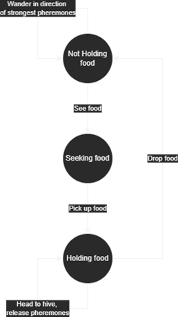
My ants ended up not being able to move in diagonals, instead they were restricted to a 2D grid; this seriously limited the models. The code these simulations use is in Appendix C and I've summarised the process here.
The process an ant follows is relatively crude (although this is not really where the problems with the model come from) and essentially involves finding which step in the model above the ant is in, and then acting accordingly.
- First, pheromone intensities need to decrease by some fraction so that when food is depleted ants do not return there forever.
- All the next steps are for each ant:
- If the ant is next to a food source (and not already holding food), then it should pick it up.
- If the ant is holding food, it should drop it if it is next to the hive, or otherwise it should move to the hive (simply matching y coordinate, then x coordinate).
- If not holding food, it should look around at pheromone levels and use or just pick randomly a direction to move.
Development
After the first 2.5 major revisions, this model did not undergo any more (much needed) development. I didn't pursue the model more because, looking back at my code, I could see that I wanted to rewrite the whole model and change how it fundamentally worked, both to remove the grid and make it overall cleaner. Doing this would have taken quite a lot of time and effort and instead of working further on the ant colony simulation, I wanted to pursue other models.
The model has three main flaws:
- Randomness, I'm not quite sure why this is, but the randomness that decides an ant's direction seriously prefers moving down.
- The grid. The ants are on a grid and this limits their movement to up, down, left, and right. It would be much better to store coordinates and a direction and have the ants move around freely in an area. Moving in diagonals on a grid would require storing past moves (unless the diagonal was exactly 45o). Removing this grid would also let ants take more efficient routes and more coherently go back and forth between food sources.
- Perhaps not a flaw in implementation, but rather my method: I underestimated the difficulty of making an ant colony simulation, which meant that I structured and wrote the code in a way that did not work well with a longer term, more complex project.
On reflection, it would have been worthwhile to continue working on this model because it would have allowed me to strengthen my conclusions and knowledge of how the model works. Fortunately, there are other examples of implementations of this I can use in my conclusions and finding these examples earlier probably would have made development easier. Removing the grid from the model would have made it easier for ants to navigate and it would have made angled paths actually shorter, which on a grid they are not. This would have made the ants more coherent and would have allowed them to behave more naturally.
Conclusion
My approach to modelling ant colonies was not very good, both from a design and implementation perspective and it does not show emergence nearly as well as some other models of ant colonies [7]. However, it does still vaguely show some of the properties we would expect to emerge from an ant colony model. I did begin revising the model so that it would be more appropriate, but I never created a fully working version.
Creating this model, I learnt a lot about how ant colonies work. Deciding what aspects of ant's behaviour to include in a model requires knowing about them in much detail and that was interesting. This model very good proof that a model of a natural system works when that model does accurately replicate the behaviour of what it's modelling. This is one of the benefits of programming these models. This model certainly furthered my aim of looking to understand the natural world using these kinds of models.
I also like the fact that models of ant colonies generally do not try to replicate all the information ants have access to and use, but still manage to replicate their behaviour very well and especially how a solution that seems only natural to programmers, e.g., using another type of pheromones to find your way back to the hive, is in fact not used in the natural world (instead ants use many factors, such as the position of the sun, an internal pedometer, and landmarks).
In nature, fireflies tend to coordinate their flashing, and people were long confused as to how such wide coordination could occur. The answer was an incredibly simple emergent behaviour which is easy to emulate programmatically [8]. The emergent behaviour of ant colonies presented a similar (although more complex) problem, and the fact that these properties can emerge from such rules is profound almost in itself.
Information
Language used: Julia
Packages imported: ProgressBars, Plots
Boids
Boids are agents which follow a few simple rules designed to simulate flocking behaviour in birds, herd animals or fish (Craig Reynolds: Flocks, Herds, and Schools: A Distributed Behavioral Model, no date).
Final Product
The goal was to introduce boids into a space and let them fly around. With the right parameters, they should exhibit flocking behaviour. Everything I did for this section was 2D. However, the same principles can (and have) been applied to 3D.
Each boid follows these 3 rules:
- Separation - don't bump into other boids.
- Cohesion - move towards the centre of mass of the boids around you.
- Alignment - match the speed and direction of boids around you.
- Keep inside the bounds of the plot.
- Keep speed under a maximum speed.
22: Under normal conditions. (80 boids).
23: With a higher vision radius (50 boids).
24: With extremely high separation.
25: With 500 boids.
Explanation
My program works by applying the functions described below in sequence as follows:
anim = @animate for _ in ProgressBar(1:steps)

    global boids

    boids = cohesion.(boids)
    boids = separation.(boids)
    boids = alignment.(boids)
    boids = keepin.(boids, w, h)
    boids = limit.(boids, speedlimit)

    boids = update.(boids, delta)

    # Pull out the x and y values to be plotted.
    x = [boid[1] for boid in boids]
    y = [boid[2] for boid in boids]

    # Plot the positions of all the Boids on a scatter graph.
    scatter(x, y, xlims=(0, w), ylims=(0, h))

end # for
Limits
Two functions are required: one to keep the boids within the edges of the plot, and another to limit the speed of the boids to some reasonable value.
"""
    keepin(boid, w, h, [edgeforce]) -> boid::Vector{Float64}

Returns the boid, with force applied to keep it inside a box
with width `w` and height `h`.
"""
function keepin(boid, w, h, edgeforce = 1)

    # Define a margin within which boids will
    # be pushed away from the edge.
    margin = 20

    #== X values ==#
    # If the boid is within the margin of the edge on the left...
    if boid[1] < margin

        # Push it right using a linear function getting
        # greater as it moves left.
        boid[3] += edgeforce * (margin - boid[1])

    # If the boid is within the margin of the edge on the right...
    elseif boid[1] > w-margin

        # Push it left using the same function.
        boid[3] -= edgeforce * (boid[1] - (w - margin))

    end # if

    #== Y values ==#
    # The same but substituting left for bottom,
    # and right for top.
    if boid[2] < margin
        boid[4] += edgeforce * (margin - boid[2])
    elseif boid[2] > h-margin
        boid[4] -= edgeforce * (boid[2] - (h - margin))
    end # if

    return boid

end

"""
    limit(boid, speedlimit) -> boid::Vector{Float64}

Returns the boid where the overall speed is capped
at the speedlimit (direction is preserved).
"""
function limit(boid, speedlimit)

    # Calculate the 2D speed of the boid.
    speed = sqrt(boid[3]^2 + boid[4]^2)

    # If the speed is greater than the speedlimit...
    if speed > speedlimit

        # Modify the velocities so that the direction
        # is the same but the speed is the spedlimit.
        boid[3] = boid[3] * speedlimit/speed
        boid[4] = boid[4] * speedlimit/speed

    end # if

    return boid

end
Separation
For separation, we simply need to find the closest boid (within the vision radius) and then push the current boid away from it using a $\frac 1 x$ function.
The lines where I update the boid's velocity require some explanation. The boid's velocity is stored with separate x and y components. However, the push function needs to know the distance to the closest boid using Euclidean distance in 2D, otherwise two boids at opposite sides of the area could be pushed away from each other since they may still have very similar y coordinates if not x coordinates. To account for this, I first find the distance to the nearest boid, and use that to determine how hard the boid should be pushed, and then split that into x and y components to be applied.
$$V_x=\frac {cS_x}S * \frac 1 S=\frac {cS_x} {S^2}$$
Here, $S$ is the total distance. Which means $\frac {S_x} S$ is the ratio between the total distance and the x displacement, or the fraction of the total displacement that is in the x direction. The same can be applied to $V_y$ by replacing $S_x$ with $S_y$. N.B., $S_x+S_y \ne S$ so the two fractions will not sum to 1.
"""
    separation(boid, [boidpush]) -> boid::Vector{Float64}

Returns the current boid with velocity changed to be pushed
away from the closest boid to it (with a 1/x relationship).
"""
function separation(boid::Vector{Float64}, boidpush = 5.0)

    # Get all the nearby boids along with how far away they are.
    n = nearby(boid[1:2], boids, vision)

    #==
	We do not want the current boid to try and avoid itself,
	so I am careful to remove it.
	==#
    n = [x for x in n if s(x[1][1:2], boid[1:2]) > 0]

    # If the current boid can see any boids at all...
    if length(n) > 0

        # Extract the distances from the list of boids and distances.
        near = [x[1] for x in n]

        # Find the location of the nearest boid.
        closest = near[findmin([x[2] for x in n])[2]][1:2]

        # Find the distance from the current boid to the nearest boid.
        distance = s(closest, boid[1:2])

        #==
        Change the velocity of the current boid by using the trip
        relationship between side lengths and the 1/distance function
        multiplied by some constant (boidpush).
        ==#
        boid[3] += boidpush * (boid[1] - closest[1]) / distance^2
        boid[4] += boidpush * (boid[2] - closest[2]) / distance^2

    end # if

    return boid

end
Here you can see the boids avoiding each other. $\frac 1 x$ is quite a strong force, so they move quite quickly.
Cohesion
For cohesion, we just need to apply a small force which moves boids towards the centre of other boids it can see. This mimics the jostling for the easy position in the centre of flocks seen in birds.
"""
    cohesion(boid, [centerpull]) -> boid::Vector{Float64}

Returns the current boid with velocity changed to be pulled
towards the centre of mass of boids it can see.
"""
function cohesion(boid::Vector{Float64}, centerpull = 0.08)

    # Initialise an empty variable that can hold [x, y] coordinates.
    center = Float64[0.0, 0.0]

    # Get the locations of the boids the current boid can see.
    near = [x[1] for x in nearby(boid[1:2], boids, vision)]

    #==
    Iterate through the list of nearby boids:
    For each boid, add the x and y coordinates to
    the x and y parts of center.
    ==#
    for b in near
        center[1] += b[1]
        center[2] += b[2]
    end # for

    # If there are any boids nearby...
    if length(near) > 0

        # Divide the center by the number of boids nearby,
        # to give an average value.
        center ./= length(near)

        #==
        Take the difference between the centre and the current boid
        and multipy that by some constant. Then apply each
        component to to current boid's velocity.
        ==#
        boid[3] += (center[1] - boid[1]) * centerpull
        boid[4] += (center[2] - boid[2]) * centerpull

    end # if

    return boid

end
Here you can see the boids forming into groups circling around the centres. As the vision radius is increased they form these groups much faster.
Alignment
For alignment, we need to find the average speed and direction (or rather, average vel'cities in x and y) and mo"""the current boid's velocity towards that.
"""
    alignment(boid, [turnfactor]) -> boid::Vector{Float64}

Returns the current boid with velocity changed to move towards
the same speed and direction of the boids around it.
"""
function alignment(boid::Vector{Float64}, turnFactor = 0.1)

    # Initialise a variable that can hold the average values.
    avg = [0.0, 0.0]

    near = [x[1] for x in nearby(boid[1:2], boids, vision)]

    #==
    Iterate through the list of nearby boids:
    For each boid, add the V_x and V_y coordinates to
    the V_x and V_y parts of the average.
    ==#
    for b in near
        avg[1] += b[3]
        avg[2] += b[4]
    end # for

    # If there are any boids nearby...
    if length(near) > 0

        # Divide the sum by the number of boids nearby,
        # to give an average value.
        avg ./= length(near)

        # Move towards the average speeds by some factor.
        boid[3] += avg[1] * turnFactor
        boid[4] += avg[2] * turnFactor

    end # if

    return boid

end
Here you can see the boids aligning with groups of other boids. You can see how some boids occasionally align with a group they can see but others are actually flung away from it; this demonstrates the need for a cohesive force.
Development
Additionally to what is described above, a few simple functions are necessary to update the parameters and to find nearby boids. These can be found in Appendix B.
Prototype
In my first prototype, the keepin, nearby, limit and update functions would remain unchanged in the final version.
In my tests, I had observed that using a 1/x function for separation would fling the boids too quickly away from each other so the effects of the other forces would be barely visible. Instead I had decided to use a sigmoid derivative. This did not work because the sigmoid derivative is not signed; it is positive on both sides, so the function could not tell from which side the boids were approaching and it would always push right/up. This also did not work because the function was not strong enough.
Despite this, the program produced not unrecognisable behaviour:
Modifications
The next steps in improving the model were changing what functions were being used for each of the different forces. I tried using an exponential at the edges for a slower turning effect. I thought this might help because it would allow the boids to be more coherent as they hit the edge. This did not help (the force was too strong). I updated the sigmoid derivative in the separation function to be signed, but this still did not fix the underlying issue which I address in the separation section above: the functions did not care about real distance between boids, only the x and y components. I also experimented with the size of the area and the number of boids to see what would be best.
In the next versions, I was still experimenting with functions in the forces. In separation, I tried using the average centre and repelling the boid from that using 1/x. In retrospect, this obviously does not make sense since this is precisely the opposite of the cohesion function. The critical realisation that I would later have is that it would be much better for me to simply repel the boid only from the single nearest boid to it.
After a few further small modifications and quality of life improvements I had produced the model described above.
I also remade the model in a game dev engine, Godot, where I was able to fiddle around with other features, such as adding different species [9] and modifying parameters live [10]. It's harder to capture their movements, but I gave a demo in my presentation.
You can find this version here.
Conclusion
Boids are a really nice demonstration of some of the properties that can be achieved with emergence. In birds and fish, we assume they flock or shoal because it is safe, i.e. they see an advantage to being together, but the boids simulations show that this kind of level of understanding is not at all necessary for flocking behaviour.
I think that boids show coordination, without communication between agents, which is essential when investigating emergent systems and when designing them. Emergent systems often emerge in the real world completely unintentionally (and without communication) and they can be both beneficial and detrimental. For example: bots setting prices by looking at prices of similar products can be emergent and this can lead to problems where items cost ludicrous amounts. Citizen-centric AIs choosing when to use electricity can lower peak grid load even if they are only designed to reduce cost to consumers. And people moving through busy corridors roughly follow fluid dynamics.
Perhaps boids was not a hugely practical application of emergence, so I could have picked something that was more practical but I think boids give a really interesting insight into bird flocking and other natural behaviours. Murmuration of birds has always been beautiful to me and others. They seem complex and hard to figure out how they work. Making this model and having a much better understanding of how these occur does not take away from the beauty of bird flocking or fish shoals, but rather adds to it. Looking at a flock of birds and understanding that each bird is likely following very simple rules, and that this effect still emerges from that, is exciting. These animals have evolved this behaviour for their own safety and of course it is simpler to follow these rules than it is to create central coordination.
The ideas that govern boids do have practical applications, trivially, in keeping animals safe, but ideas of group motion and coordination have also been applied in robotics, physics, and search optimisation techniques (Boids (Flocks, Herds, and Schools: a Distributed Behavioral Model), no date) [11]. It is interesting to compare the ant colony model to boids, since they are both biomimicry which coordinate many agents. Boids do not have any centrally aligned goal, but ants do have that built into how they work, despite this they both exhibit coordinated behaviour.
I made some silly mistakes in my initial boids simulations, so I am glad I came back to the project when I had a break in progress in my plan which I had allocated as time to finish up aspects of models that needed extra work, to produce the polished model above.
Information
Language used: Julia, and GDScript for Godot
Packages imported: ProgressBars, Plots
Reaction Diffusion
This simple (albeit slightly unrealistic) spatial simulation of a chemical reaction demonstrates the unpredictability of making very small changes to the starting conditions of a chaotic system (that may be emergent) and shows how lifelike structures can emerge on a larger scale than where they are applied.
Final Product
A Reaction diffusion simulation is a simulated reaction between two chemicals, A and B. Four steps happen every tick of the reaction:
- A and B diffuse a little into their surroundings.
- Two Bs and an A can react to form three Bs (BBA -> BBB).
- Some A is added.
- Some B is removed.
The simulation works by approximating the chemicals in a grid of cells each of which contains between 0.0 and 1.0 of A and the same of B representing the portion of the total max A or B that can fit in each cell.
When these rules are applied, we can see myriad different emergent behaviours by plotting the amount of A:
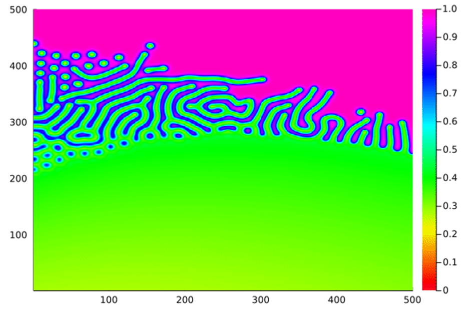
26: Varying the feed rate along the x axis and the kill rate along the y axis.
27: Growth (network): Feed = 0.055, kill = 0.062.
28: Growth (without connection): Feed = 0.05, kill = 0.065.
29: Mitosis: Feed = 0.05, kill = 0.066.
Explanation
The model creates a gif of the reaction by capturing every 40th iteration and playing it back at 30 fps.
# For each relevant frame in the cache...
anim = @animate for frame in ProgressBar(cache.A)

    # Create a heatmap showing the amount of A.
    heatmap(frame, clim=(0,1), c = :gist_rainbow)

end # for

# Great a gif of all the heatmaps.
gif(anim, "reaction"*string(loop)*".gif", fps = 30)
Initialisation
The initial state and properties of the simulation are particularly important in this case. I use a number of starting patches of B. If there is any order in these placements, then this order is generally shown at the end of the simulation so I use random placement. This has been quite effective at creating organic structures.
# Constants
dims = 200
steps = 1000
interval = 40

# Variables for storing the state.
A = ones(Float64, dims, dims)
A2 = ones(Float64, dims, dims)
B = zeros(Float64, dims, dims)
B2 = zeros(Float64, dims, dims)

# Seed B
for _ in 1:dims
    B[max(1, trunc(Int, rand() * dims)), max(1, trunc(Int, rand() * dims))] = 0.9
end # for

# Setup caches
cache = (A = [zeros(Float64, dims, dims) for _ in 1:trunc(Int, steps/interval)],
         B = [zeros(Float64, dims, dims) for _ in 1:trunc(Int, steps/interval)])

# Global constants
global feed = 0.055
global kill = 0.062
global D_A = 1.0
global D_B = 0.5
global delta = 1.0
Diffusion
For diffusion, we need to find some function that will get the amount of a chemical after diffusion that won't change the total amount of a chemical after this has been applied to all cells. For this I used a Laplacian function which calculates where we would expect fluid to collect in a field.
"""
    diffuse(coords, C) -> Float64

Returns the amount of chemical C (where `C` is a 2D matrix)
at `coords` after some diffusion.
"""
function diffuse(coords::Tuple, C)

    #weights = [[0.05, 0.2, 0.05], [0.2, -1.0, 0.2], [0.05, 0.2, 0.05]]

    #==
    In order to calculate the new value for this cell:
    Create a weighted average of all the cells around it,
    (orthogonally adjacent cells have a weight of 0.2 and
    diagonally adjacten cells have a weight of 0.05).
    Then subtract the value in the current cell.
    If any of the adjacent cells don't exist, assume
    they have the value of the current cell.
    ==#
    return sum(
        get(C, (coords[1] + 1, coords[2]), C[coords[1], coords[2]]) *0.2 +
        get(C, (coords[1] - 1, coords[2]), C[coords[1], coords[2]]) *0.2 +
        get(C, (coords[1], coords[2] + 1), C[coords[1], coords[2]]) *0.2 +
        get(C, (coords[1], coords[2] - 1), C[coords[1], coords[2]]) *0.2 +
        get(C, (coords[1] + 1, coords[2] + 1), C[coords[1], coords[2]]) *0.05 +
        get(C, (coords[1] - 1, coords[2] + 1), C[coords[1], coords[2]]) *0.05 +
        get(C, (coords[1] - 1, coords[2] - 1), C[coords[1], coords[2]]) *0.05 +
        get(C, (coords[1] + 1, coords[2] - 1), C[coords[1], coords[2]]) *0.05 +
        get(C, coords, 1.0) * (-1.0)
    )

end
Simulation
Storing all the data from long simulations requires too much memory, so I break the whole task up into fragments each of which generate a gif and then I can stitch those together to get the whole simulation.
Since the A and B values are between 0 and 1, they lend themselves nicely to being treated as probabilities. If the amount of A is 1.0, then we are certain to be able to find some A to react, but if there is only 0.1 B then very little reaction will occur, because 2 Bs are required. In this vein, we use ABB as the amount of A that will react and become B.
To calculate the new amount of A at a coordinate we use the following:
$$A_{x,y}^{'}=A_{x,y}+(D_A \nabla \cdot A_{x,y} - A_{x,y} B_{x,y}^{2}+F(1-A_{x,y}))\delta t$$
Where DA is some constant (1.0), $\nabla \cdot A_{x,y}$ is the diffused $A$ value, $F$ is the feed rate and $\delta t$ is the time interval. $A_{x,y} B_{x,y}^{2}$ is the amount of A that is going to react (and become B, so it is subtracted). F is multiplied by $(1-A_{x,y})$ which prevents $A_{x,y}$ from ever going over 1.
To calculate the new amount of B at a coordinate we use the following:
$$B_{x,y}^{'}=B_{x,y}+(D_B \nabla \cdot B_{x,y}+A_{x,y} B_{x,y}^{2}-(K+F) B_{x,y})\delta t$$
Where DB is some constant (0.5), $\nabla \cdot B_{x,y}$ is the diffused B value, F is the feed rate, K is the kill rate and $\delta t$ is the time interval. In this case, $A_{x,y} B_{x,y}^{2}$ is added because the A becomes B. $(K+F)$ is multiplied by $B_{x,y}$ so that $B_{x,y}$ never goes below 0 and so that the amount that is removed is proportional to the amount that is present.
# Looping in order to break up the task.
for loop in 1:20

    # Iterate for 'steps' many steps...
    for i in ProgressBar(1:steps)

        # Disambiguate access to A and B we defined above
        global A
        global B

        # For each x coordinate (columns)...
        Threads.@threads for x in 1:dims

            #kill = 0.05 + x/dims * 0.02

            # For each y coordinate (now rows)...
            # This therefore goes through every cell.
            for y in 1:dims

                #feed = 0.04 + y/dims * 0.04

                # Calculate the amount of ABB which will become BBB.
                ABB = A[x, y]*B[x, y]*B[x, y]

                #==
                Calculate the amount of A that should be at these coordinates
                and store it in A2 (so that all the new values are calculated
                before the old ones are used).
                ==#
                A2[x, y] = A[x, y] + (D_A * diffuse((x, y), A) - ABB
                           + feed * (1 - A[x, y])) * delta

                # Do the same for B.
                B2[x, y] = B[x, y] + (D_B * diffuse((x, y), B) + ABB
                           - (kill + feed) * B[x, y]) * delta

            end # for
        end # for

        # Store the current frame in the cache.
        # The chop is used to not store only necessary frames.
        chop = trunc(Int, i/interval - 1/(interval + 1)) + 1

        #==
        Since arrays are just pointers in julia, a copy
        is created so that when A2/B2 is modified later it
        does not also modify the cache.
        ==#
        cache.A[chop] = deepcopy(A2)
        cache.B[chop] = deepcopy(B2)

        # Update A and B with their new values so that
        # the next iteration can run.
        A = cache.A[chop]
        B = cache.B[chop]

    end # for

    #== ANIMATION ==#

end # for
Development
A reaction diffusion simulation like this is particularly well suited to being run on a GPU. This is because each individual calculation per cell is very simple, but there are hundreds of thousands of those calculations to do each tick. GPUs have many individual cores which can perform simple calculations. However, these cores are not very powerful, since computational poweris not a bottleneck for this kind of program a GPU is particularly suited to running it quickly. A CPU has a small number of more powerful cores which makes it less efficient at running a simulation like this. Realising this, and not wanting the simulations to take too long to run, I initially wanted to write this simulation in C++ using OpenFrameworks. However, I did not have enough time to learn C++ or OF; instead, I used Julia which runs on the CPU as I have for my other projects (there is some GPU support for Julia but it is in development for the GPU architecture my computer uses).
Prototype
Very little changed between my initial prototype and final product. Some time was spent making sure the algorithm was efficient and produced GIFs that were at a watchable pace. The most time was spent experimenting with values and starting conditions to see what different effects the program could produce. This is also why varying the Feed and Kill values across the axis was particularly useful - it allowed me to pick on areas of particular interest and expand on them.
30: (F = 0.055, K = 0.062) The first simulation I saved.

31: (Varying F along x-axis and K along y-axis) See how the starting conditions matter (this simulation misses a lot of the disconnected areas because there were no seeds there. It is also defined by the line of a seed, which is not useful for finding area.
32: (Varying F and K in the same way) This product is defined by the horizontal lines of the seeds.
Conclusion
Reaction diffusions are a different kind of emergent system to the others I've shown because there are not really individual agents like there were boids or ants in the other models, since each cell is not mimicking an organism but is instead just a fixed point on a grid where a rule is applied. You could say this model mimics physics rather than biology. This difference is what makes it a model worth paying attention to when trying to understand the practical applications of emergence. Intelligent behaviour is much less obvious here because there are no agents taking actions we can relate to, but the emergent behaviour in fact occurs at a much larger scale than individual cells and is shown by results that are very lifelike and unusual. Reaction diffusion simulations certainly meet the requirements for emergence due to the unpredictability of their results alone.
This model was generally very simple to code and produced very enjoyable results. It is a shame that the scope of simulations was severely limited by the fact I was running the code on the CPU, whereas the GPU would have been very well suited to a task like this. Some simulations I've seen online have been done to a much larger scale and when this is combined with the idea of varying the parameters over the area, you can see a much greater degree of specificity and individual types of behaviour caused by the different parameters.
Making this model, I learnt about how properties can emerge on a much larger scale (fig 27, for example, is on a 600x600 grid, which means for each step you need to calculate 360,000 cells, and we can see each band must be ~10 cells across) without having discreet agents acting or moving around. The most thorough version of this model (U-Skate World, an Instance of the Gray-Scott System at MROB, no date) I could find classifies it as a class 4 cellular automata, which means that "Nearly all initial patterns evolve into structures that interact in complex and interesting ways, with the formation of local structures that are able to survive for long periods of time." ('Cellular automaton', 2022). I agree with this claim as we can see from my examples that changes in one place can affect a large area, and that the structures are complex and interesting. Like Conway's Game of Life (Life) (probably the most famous cellular automaton), the behaviours we see are totally unexpected. Life has been shown to be Turing complete (Turing machine - LifeWiki, no date), and Wolfram has claimed that many class 4 cellular automata are Turing complete, although a stricter definition would be required to show such a thing, that's very surprising to me and it shows the complexity (or unpredictability almost) of the final properties of this emergent system. This model has helped me quantify the level of complexity in some emergent systems and understand how emergent properties can emerge at a much larger scale than the individual agents.
Information
Language used: Julia
Packages imported: ProgressBars, Plots, ColorSchemes
Machine Learning
Final Product
My neural network follows a simple loop: take the past letters, and predict the next one, then get the cost of the predictions (relative to if they had been 100% correct) and compute the gradients of the parameters with respect to the cost function and update our parameters using gradients descent. The way it does this is emergent, because it uses a collections of nodes which each perform a simple task.
Explanation
A neural network is a collection of neurons, or nodes, which are attached to some or all of the nodes in the previous layer via some maths which determines how much of a priority each of those inputs are. Whenever you want an answer from the network, you provide the inputs and read the outputs that are generated by propagating through a number of layers like this. There is nothing inherently complicated or unique (fundamentally at least) about the architecture of a neural network - it's those weights and biases that decide whether a NN plays chess totally randomly or if it can beat Carlsen [12].
Unfortunately for us, finding those ideal numbers is really difficult. So that's where training comes in: we initialise the NN with a set of random weights and biases and then forward propagate through it to find what it predicts for each of our sample inputs. Then we can work out how far the guesses were from the real answers and in what directions, using this information we can move the numbers in the NN slightly towards values which will give the correct outputs by moving backwards through the NN or backpropagating.
There are other ways of training neural nets, including introducing some element of random variation and training two networks to compete against each other to remove the requirement for prelabelled data, but the fundamental principles still apply.
main.jl
Here the data in data.txt is processed to be inputs into our neural net. It takes each line and splits it into 15 character long chunks (with overlap, and allowing blank characters at the beginning).
Take for example:
AG v Wilkinson -- Ahmad Ors
First we make each character in the string into an array with one 1 showing the character so A would generate an array like
Int[..., 0, 0, 1, 0, 0, ...]
Each value in the array is a specific character, with a special character at the end for stop.
Let us assume our input length is 5 characters; this is like the NNs memory. To create the first datum for our NN, we add 4 (input length -1) blank arrays and the array we just generated (flattening all of these as we go). For the next character, we add 3 (input length -2) blank sets A and then the array for G. Once we reach 5 characters in the string, we remove characters so that it only sees the last 5. For example datum 6 would be "G v W".
This gives us a lot of data points which we can use as training data. So we can pass that (as DMatrix) but we need some other parameters first:
function train_network(layer_dims::Vector{Int64}, DMatrix::Vector{Any}, Y::Vector{Any}; η = 0.001, epochs = 500, seed = 1337, verbose = true)
layer_dims looks something like this:
Int64[345, 207, 207, 207, 69]
Where each value describes the number of neurons in a layer of the NN (the first and last layers describe the input and output layers respectively). layer_dims is a hyperparameter, which means that if we wanted to optimise the NN (and had lots of resources) we could train the NN using some kind of algorithm that worked out how many layers we need (we want to minimise layers where we can, to avoid doing extra calculations, but we don't want to have so few our model can't be accurate). The lengths of the layers are arbitrary, but the input layer must match (in our example it's 5∗69=345) the length of the arrays in DMatrix and the output layer must match the length of the arrays in Y.
Y is the set of the actual values from our dataset for each item in DMatrix. We have been calculating these alongside our inputs so that the two vectors line up. It's the next character in our string (because that's the one we want the NN to guess).
train.jl
This contains the function train_network which I briefly talked about above which outlines the steps my NN is going to take to learn. η describes the learning rate (more on this later!). epochs tells our code how many times to go through the whole training dataset. seed is used instead of the default Random Number Generation (RNG) so we get consistent results (useful to recreate situations). verbose tells our code whether it should print to console as it does things.
First we have to initialise our model, and for this we use initialise_model(layer_dims, seed) which can be found in...
initialise.jl
function initialise_model(layer_dims, seed)
This function creates and returns a dictionary params which contains all the initial weights and biases for the model. The biases start at 0, but the weights are randomised to avoid symmetry (we want different parts of our NN to learn to do different things but if the weights all start the same, they would never be different so there might as well only be one neuron in each layer).
The next thing to do in train.jl is to start running our NN! First we propagate forward through the model in...
forward_propagation.jl
forward_propagate_model_weights(DMatrix, params) loops through each layer of the NN and gets the values:
For layer l:
$$Z_{l,n}=W_{l,n} A_{l-1}+b$$
So for each neuron in each layer (except the input layer) we multiply each value in the previous layer by some number (specific to each neuron), and then add a bias (find this in linear_steps.jl). We're not quite done there for each layer. We actually need to apply an activation function so to restrict the results. This also adds mathematical complexity to the network, which allows it to reach solutions with more detail. The most important activation function is the one in the final layer (in the other layers I primarily use tanh). In the final layer we use a softmax activation function to obtain values above 0 which sum to 1, like probabilities.
$$A_{l,n}= \frac {e^{-Z_(l,n) }} { \Sigma {e^{-Z}} }$$
The greater $Z$ is, the closer this will be to 0, and the smaller $Z$, the closer to 1. Usefully, it can never fall outside of those bounds (find activation functions in activations_functions.jl).
Now that we've iterated through our NN, we need to calculate the cost of our results in...
cost.jl
For now I use an implementation of binary cross entropy which says that if you have two functions $p(x)$ and $q(x)$ you can calculate the distance between the results of the two functions essentially like this:
$$C=q(x) \log_2 \left( \frac 1 {p(x)} \right)$$
The derivation for this is quite complicated but a very readable explanation can be found in (Visual Information Theory -- colah's blog, no date). I do not know whether or not this is the correct cost function for this NN, but it should be close enough that it doesn't matter (in many ways, that is a guiding principle of machine learning).
Our implementation of this looks slightly different:
$$C = \frac {-\Sigma (Y \log_2 \hat Y +(1-Y) log_2 (1-\hat Y))} m$$
Where $m$ is the size of $Y$. This actually gives us the same thing because our actual values ($Y$) are binary. When the correct value for that neuron of the sum is 0, the sum can be simplified to:
$$1 * \log_2 (1-\hat Y)$$
This is almost the same form as above. We've got $1-\hat Y$ rather than $\frac 1 {1-\hat Y}$. I've accounted for this by taking that out as a minus (simple log laws). This affects every term, so I took it out of the sum. A similar thing is obtained if $Y$ is 1:
$$1 * \log_2 \hat Y$$
Next, we need to do the really interesting bit: actually learning in...
backpropagation.jl
We can think about this quite clearly if we imagine a neural network with only one neuron per layer. Essentially we need to take the value we got and modify our NN to produce a value that's slightly closer to our desired value. Let us take a neuron, n, it has a weight, w, and bias, b. It received an input (A) 0, and we want it to output 1. We know the output we got, Y_n, and the output we wanted Y ̂_n.
$$\hat Y_n=wA+b$$
It's easy to see how we could optimise one neuron to create the result we want. Substitute for A and our desired $Y_n$. e.g.
$$1=0w+b$$
Picking random values for $w$ and letting $b = 0$ initially (as we do in our NN) currently gives us:
$$0*0.74 \ldots +0=0$$
We can clearly see that $w$ does not affect our result in this case [13], so we can modify $b$ only:
$$b=b+(Y_n-b) \eta ;$$
Where $\eta$ is the learning rate.
$b=0+(1-0)*0.01=0.01$
So we've modified our value of $b$ to give a slightly better answer than before. We could let $\eta =1$ then the NN would correctly guess the right answer for this situation! However, this is called overfitting and doesn't actually solve the problem we want it to. Our NN would always be completely overhauled each time we backpropagate to get the ideal result, but we would never converge on something which could produce an accurate result from data it hasn't seen before (or even from other data in our dataset, if $\eta = 1$). Even in less extreme cases, overfitting is still a big issue. If your NN learns for too long it may learn to fit perfectly to your data and unlearn how to solve the problem which means it would produce less accurate results when it sees data it's never seen before! (This is also why it's important to keep some data for unsupervised tests after supervised training.)
The partial derivatives of each of the cost function with respect to Y can be calculated as follows:
$$\frac {\delta C} {\delta \hat Y }=\frac {-Y} {\hat Y} + \frac {1-Y} {1-\hat Y}$$
Now that we have this value, we can feed it back into the last layer of neurons to calculate the actual values of $\delta W$, $\delta b$, $\delta A$ (or, more accurately, the gradient at the tangent to the point on the curve where each parameter lies). This process can then be repeated for each layer backwards (using the $\delta A$ instead of the $\delta \hat Y$ value). So using these calculated gradients for all of the layers, we can update the parameters by moving slightly downwards along each gradient in gradient_descent.jl.
Final steps
The final step is to log all of the parameters and the results of the neural net training.
Then this loop repeats with the new parameters, each loop aims to move the parameters slightly closer to the correct answer each time. After all the loops are done, we can return the important parts of the neural network for use in unlabelled data/in the real world.
Development
Code snippets can be found in Appendix D.
Prototype
The prototype was not particularly smartly made and it barely worked. However, it was a very important step in production from where I could improve. Initially I was using reLU functions in all of the hidden layers, which I changed later.
Modifications
Most of my modifications were: debugging, testing and implementing new ideas. In summary: I made significant progress and learnt a lot but I did not produce a neural network which could really demonstrate completing a task like mimicking human text in a complex way (although I can still demonstrate it).
The first change I made was to prepare and begin testing new activation functions: tanh and softmax (for final layer) rather than reLU and sigmoid, which I was using previously. This involved working out the derivatives for these functions too and implementing those. It took me a longer than expected to work out why these activation functions weren't working as expected or were giving errors.
First off, I was getting errors because there was some notation I wasn't using correctly in my code and I was using floating point values when iterating through the neural network; sometimes those would become so tiny they would become 0 which would cause errors in division (specifically in the softmax function, e^(-x)/(Σe^(-x) ) where the sum would become 0). I also encountered the opposite problem of dividing by infinity. [14]
To solve these issues, I decided to limit the weights and biases to 100/1,000/10,000 (I changed the value I used but these would all do the job) because at that point, once passing through tanh, the value will be so close to 1 or -1 it doesn't matter whether it's 10,000 or 10,000,000. I also had to use BigFloats, which seriously slowed down my code, but resolved a number of issues. These values allow Julia to manage arbitrary precision in the back end so tanh (for example) will never give a value of 1. and values will never tick over to 0, even when they are much smaller than a Float64 could handle. I sped up the code a lot by reducing the data size and the network size, so this didn't end up being an issue.
I did realise that this was actually a common problem when using activation functions like tanh called Exploding Gradients, where the derivatives of the functions become huge because even massive changes only affect the activated output a tiny amount and the net was trying to make some values closer to 0 and some closer to 1.
Then I went through the data and cleaned it up to remove all punctuation (except -) and numbers and upper/lowercase letters (this change made in code not in data.txt). This makes the net's job easier and means less training data should be required to get a good result.
Next, I added a logging system which creates files containing all the predictions the net has made and the parameters of the network which I could then analyse later. These would allow me to see if the network was doing its job and observe any obvious problems in the parameters. The logs remain on my computer at home, where I have been able to run all the tests I have required.
A significant change I then made was that I fully vectorised the whole process of training. Previously, I would forward propagate for one data point, then go calculate the gradients and backpropagate for that one point, then move on to the next, but this is inefficient compared to the new approach of forward propagating for all the points and then calculating gradients for all the points, then only updating the model weights once. Not only is this more efficient but it also helps the net train because it will have no preference towards the most recently seen data point as it sees every point at once.
This vectorised process also allowed me to make the program threaded. Using 4 threads rather than one significantly (doubled ish) the speed of the program. Threading essentially takes one process which you want to do a lot of times and distributes each task between different threads, which will usually run on individual Cores on the CPU. There is overhead managing the threads, which means you don't get quite the expected increase in speed (e.g., 4x off 4 cores is not possible) but the speed up is still significant.
I did some further data cleaning to hopefully confuse the neural net less. (removing random leading '-' which had appeared and I wasn't sure why, but they weren't supposed to be there). This is a hugely important process and not having good data is the main reason neural networks fail to do what you want. They will do exactly as you ask, which may not be what you want.
I had been running a lot of (very small) tests throughout this process and I have logs for most of them. It was not able to replicate human names or the structure of these cases. The most important next step for me is to get the Swish activation function working. It seems like it would be very appropriate for the task and is quite exciting.
Later in development I changed the limits on layers using tanh to 3. This seems to be a more normal value in Machine Learning.
Conclusion
I'm very glad I pursued a machine learning model as part of this EPQ but there are certainly some things I would have done differently if I were to do it again, and some further improvements I would like to make. I think it would have been good to pick a simpler task for my neural network, like playing a simple game or generating a more obvious sequence. It definitely would have been better to work on machine learning as one of my final projects rather than my first. If I'd had more time to work on this, firstly, I would get the swish activation function working. I'd also tidy up some of the mess to do with datatypes in my code, which exists since I was less familiar with matrices in Julia when I made this. Ideally, I would like to try using some prebuilt machine learning modules for Julia (or python) which would likely let me make a lot of progress more quickly.
The results I got from this model, while far from ideal, were actually good at demonstrating both emergence and some classic problems with machine learning. In general, the model would very quickly realise that the best way to minimise the cost function is to assign all of the probability to one letter, which just happened to always be 'A' or 'B'. Somewhere around here the AI found a local minima in this situation which was a result of the cost functions and activation functions (tanh) I was using not being particularly well suited to the task. Interestingly, although the NN was always guessing A or B with the most confidence, it had assigned up to 15% likelihood to the correct character after enough learning. Local minima are a big problem in Machine Learning, and there are a number of methods for dealing with them, the fundamental problem is we want to find the best solution, so we want the global minima. If the curve is very lumpy, you might get stuck in a local minimum instead and, since the whole point is we don't know what the curve actually looks like, never know if you've reached the true minimum.
Information
Language used: JuliaPackages imported: DataFrames, CSV, Dates, ProgressBars
Conclusion
Throughout the production of my EPQ, I have created programs to model emergent behaviour to varying degrees of success. The ACO, Boids and Reaction-diffusion experiments have been the most obviously successful, with the Machine Learning perhaps teaching me the most. I set out to learn more about potential applications of emergence in the real world, as well as natural situations emergencecan model simply as a demonstration of how powerful the system is.
Machine Learning and artificial intelligence get thrown around a lot as fancy modern things which are often poorly understood, but which seem to pop up everywhere and, to some extent, this is the case. Even the architect of a complex neural network does not understand what each neuron does or how it came to be, and this means that any bias in datasets can result in an AI that doesn't answer the question we wanted it to (but rather the question we asked). For example, dataset bias is what teaches Ais, which screen job applicants, to be racist and it can be very hard to eliminate this from our datasets, but that just shows how ingrained racism is in our own society. The datasets are real ones, created by humans after all. People really do understand how machine learning works, just perhaps not a specific NN is doing. Researching machine learning and building a neural net for this project also taught me that it is not the AI's fault when it falls into a trap like this, as machine learning models only reflect the data they were given. As with the other models I created, it is a fundamentally simple system (it only seems complex because it benefits from a certain level of mathematical complexity).
The boids, reaction-diffusion, and ant colony models are all about biomimicry (because of course, biology has no central intelligence so of course it would create systems with beautiful emergent properties to solve complex tasks). Watching the boids fly around and enjoying changing the numbers that govern their individual behaviour is an enthralling process. The same is true for the reaction-diffusion model. The mere fact that we have described such simple systems that, when applied consistently, have such surprising and splendid effects is in itself awesome enough to warrant their investigation.
It is clear to me that there is a lot of potential for emergent systems to solve problems in the real world, for example allowing for something akin to central control without any of the limitations which that entails. We are already seeing some of the implications of Machine Learning being realised, for better and for worse; every user of services like Netflix can get personalised recommendations without a human ever having to figure out a user's likes and dislikes. (This is being pushed further and further. The "YouTube Algorithm" has been succeeded by an even better tuned algorithm powering TikTok's recommendations). I am very excited to see where the world takes emergence.
Emergence is very much worth continuing to investigate - it is what turns proteins to cells, cells to people, and people to societies (Emergence - How Stupid Things Become Smart Together, 2017). It is absolutely necessary for all life and practically everything we know. As society moves on to create new things, emergent behaviour will follow, as it always does, and it would be much better if we used that intentionally to our benefit rather than accidentally to our detriment.
Glossary
- Algorithm - A series of steps which will always find the exact solution to a particular set of problems.
- Heuristic - A method of generating solutions to problems which aren't guaranteed to come up with the best solution, but provide an approximation, which can be trusted to some degree. They might use randomness or some algorithm which solves a simpler problem to create an imperfect solution.
- The Travelling Salesperson Problem - A problem to find the shortest loop a merchant should take through a set of cities.
- Exponential - A function where increasing the input by some value increases the output by a constant factor. They have equations of the form y=a^x.
- Brute Force - A method of problem solving where all the possible answers are tested to find the best one.
- Heatmap - A graph which shows a grid where each grid square has some value represented as a colour (colour legend to the right of the graph).
- Biomimicry - Mimicking nature in programs (or as solutions to problems e.g. in architecture).
- Matrix/Vector - A Vector is a list of values. A vector can even store vectors! Whereas a matrix is a like a coordinate grid of values (in n-dimensions).
- Line/Segment - A line is an infinite line that can be defined by extending the line between two points. A segment is a finite section of a line, e.g. the section between two points.
- Colinear - All lie on the same straight line.
- Euclidean Distance - Distance between points how we usually perceive it - as measured with a ruler between two points or using Pythagoras' theorem.
- GPU - Graphics Processing Unit which is much like the CPU, but it is good at performing many simple operations at once, like those necessary to display an image.
- Initialise - Create or ready something for use.
- fps - Frames Per Second.
- OpenFrameworks - An open-source framework for writing GPU calculations in C++.
- Tanh - An S shaped function with horizontal asymptotes at -1 and 1.
- Softmax - A function that takes any values and maps them to a fraction of the total using e^(-x).
- Datum - A single piece of data or a part of data.
- Hyperparameters - Parameters that affect the whole model and are changed to find the optimal way to run it.
- Dictionary - A collection of keys with corresponding values in which keys can be looked up to get/set their values.
- Debugging - A process of removing issues (or bugs) from a program.
- Quality of life (improvements) - A quality of life improvement is a change that doesn't really affect the code or method fundamentally and instead makes it easier to use or interpret the result. E.g., plotting graphs to make the results clearer or organising code to make it easier to change and understand how it works.
Literature Review
My main method of ensuring that sources were rigorous and accurate was through testing. I could implement a source's ideas in my model to see how well it performed. This was most difficult with my machine learning model, where it was sometimes unclear if an idea had worked or not. To find sources, I would generally follow links around sources that I had already seen to be thorough, and I tended to prefer more recent work.
Emergence in general
Sebastian Lague's videos and physarum both gave me good jumping off points since they had peaked my interests.
Relevant sources:
- (Emergence - How Stupid Things Become Smart Together, 2017)
- (Emergent Intelligence - Chetan Surpur, no date)
- (physarum - Sage Jenson, no date)
- (Sebastian Lague, 2021)
Ant Colony Optimisation
I found some examples of ant colony optimisation for this problem (Dodd, 2020; Dent, 2021). I found Dent useful because it showed the method in practice and the different parameters I would need to use to have a working model. Dodd was useful because I was able to use their code to understand how the greed system worked. Initially I saw an application of ACO in (Sebastian Lague, 2021). I went on to find a slightly more thorough explanation of the heuristic which was useful for my implementation (Eddie Woo, 2015).
Relevant sources:
- (Eddie Woo, 2015)
- (Dodd, 2020)
- (Dent, 2021)
- (Sebastian Lague, 2021)
Ant Colonies
I didn't use any code examples when developing this (which was a mistake), as I thought I had a good understanding from (Emergence - How Stupid Things Become Smart Together, 2017; softologyblog, 2020; Sebastian Lague, 2021).
Relevant sources:
- Emergence - How Stupid Things Become Smart Together, 2017
- softologyblog, 2020
- Sebastian Lague, 2021
Boids
I initially was given the idea to investigate boids in (Sebastian Lague, 2019) which led me somehow to this paper (Craig Reynolds: Flocks, Herds, and Schools: A Distributed Behavioral Model, no date) and this code/website (Eater, 2022, no date). There are plenty of implementations of boids online, but they all do similar things to Eater, so they weren't worth referencing when programming my model.
Relevant sources:
- Sebastian Lague, 2019
- Eater, 2022
- Craig Reynolds: Flocks, Herds, and Schools: A Distributed Behavioral Model, no date
Reaction Diffusion
I initially found out about reaction-diffusion simulations through (physarum - Sage Jenson, no date). From there I found (Reaction-Diffusion Tutorial, no date) with an explanation of the simulation and (U-Skate World, an Instance of the Gray-Scott System at MROB, no date) which demonstrated some of what could be achieved at a large scale. I was also inspired by Sebastian Lague's showcase of emergent models (Complex Behaviour from Simple Rules: 3 Simulations, 2021). It was difficult to find work (other than Slackermanz) on multi-neighbourhood cellular automata, as most work was on Conway's Game of Life. This is part of the reason why I didn't pursue a multi-neighbourhood cellular automata model.
Relevant sources:
- Cristina, 2021
- 'Understanding Multiple Neighborhood Cellular Automata - Slackermanz', 2021
- physarum - Sage Jenson, no date
- Reaction-Diffusion Tutorial, no date
- U-Skate World, an Instance of the Gray-Scott System at MROB, no date
Machine Learning
I wanted to pursue machine learning for this project when I was reading (Shane, 2020), which is entertaining and informative. This model required a substantial portion of this project's research, but two foundational articles were: (Andrade, 2019; Brenyah, 2020). These provided the vast majority of the code and structure for the neural network which was otherwise beyond me. I also used (Serengil, 2017; Refaeli, no date; Tung.M.Phung, no date; 12 Types of Neural Networks Activation Functions: How to Choose?, no date; Visual Information Theory -- colah's blog, no date) to provide additional explanation and methods. Colah's blog was very useful in gaining the necessary understanding of information theory and sources about Activation functions generally provided useful guidance in deciding which functions to use. Andrade and Brenyah both gave useful structure to the project and plenty of the code, but I did have issues with the methods in each of them; I had to combine and refine their ideas for example in the layout and structure of the training function. I felt many data should be tested before performing gradient descent, which was not how they had implemented it.
Relevant Sources:
- Serengil, 2017
- Andrade, 2019
- Brenyah, 2020
- Shane, 2020
- Refaeli, no date
- Tung.M.Phung, no date
- 12 Types of Neural Networks Activation Functions: How to Choose?, no date
- Visual Information Theory -- colah's blog, no date
Appendix A
Additional code for Ant Colony Optimisation.
"""
	gen_points(n::Int, dims::Int) -> Vector{Vector{Float64}}
Returns `n` points in `dims` dimensions.
"""
function gen_points(n::Int, dims::Int)
	return [[rand() for _2 in 1:dims] for _ in 1:n]
end # function

"""
	s(a, b) -> Float64
Returns the euclidean distance between two n-dimensional points, `a` and `b`.
"""
function s(a, b)
	@assert (size(a) == size(b))
	return sum([(a[i] - b[i])^2 for i in 1:length(a)])^(0.5)
end # function

"""
	draw(points, order, [f])

Plot the route `order` through `points`.
"""
function draw(points::Vector{Vector{Float64}}, order::Vector{Int}, f = "route.png")

	# Extract the x and y values for plotting.
	x = [points[i][1] for i in order]
	y = [points[i][2] for i in order]

	# Plot.
	plt = plot(x, y, xlims=(0, 1), ylims=(0, 1), marker=:cross, title=string(length(points)) * " points")

	# Save as a .png.
	png(plt, f)

end # function

function draw(ph::Matrix{Float64})

	plt = heatmap(ph)
	png(plt, "route_ph.png")

end # function
Appendix B
A small function is used to update the positions of the boids according to their velocities (after all the other calculations have been done).
function update(boid::Vector{Float64}, delta)

	# Boid position is the current position (in components)
	# plus the velocity * some time interval.
    return [boid[1] + boid[3] * delta, boid[2] + boid[4] * delta, boid[3], boid[4]]

end
A function to calculate the distance between two points. This applies Pythagoras's theorem in n-dimensions.
function s(a, b)
    @assert (size(a) == size(b))
    return sqrt(sum([(a[d] - b[d])^2 for d in 1:length(a)]))
end # function
A function to find the boids nearby to a point (works in any number of dimensions).
"""
Returns an array of all the boids within a radius r about centre c.
"""
function nearby(c, boids, r)
    return [(b, sqrt((c[1] - b[1])^2 + (c[2] - b[2])^2 )) for b in boids if sqrt((b[1] % w - c[1])^2 + (b[2] - c[2])^2) <= r]
end

function nearby(c, boids)
    return [(b, sqrt((c[1] - b[1])^2 + (c[2] - b[2])^2 )) for b in boids]
end # function
Additionally some setup is required:
using Plots
using ProgressBars

theme(:dark)

#== FUNCTIONS HERE ==#
# Initialise constants

# Create n boids in random locations including
# just outside of thet bounding box.
boids = Vector{Float64}[[rand()*3/2*w-w/4, rand()*3/2*h-h/4, (rand()-0.5) * 5, (rand()-0.5) * 5] for i in 1:n] # x,y,dx,dy

#== ANIMATION HERE ==#

gif(anim, "boids.gif", fps = 40)
Appendix C
Here is the code used to create the simulations shown (or at least a very similar version was used). (This is not good code)
using Plots
using ProgressBars

steps = 200
dims = 100
ants = 200
wander = 0.5
speed = 1
global dirs = [-pi/4, 0, pi/4]

ph = zeros(Float64, dims, dims)
ant = Vector{Float64}[Float64[dims/2, dims/2, rand()*2*pi] for _ in 1:ants]
prev_ant = Vector{Float64}[Float64[dims/2, dims/2, rand()*2*pi] for _ in 1:ants]
holding_food = fill(false, ants)
food = zeros(Float64, dims, dims)
space = fill(true, dims, dims)
hive = [trunc(Int, dims/2), trunc(Int, dims/2)]

food_cache = [zeros(Float64, dims, dims) for _ in 1:steps]
ph_cache = [zeros(Float64, dims, dims) for _ in 1:steps]
ant_cache = [zeros(Float64, dims, dims) for _ in 1:steps]

# Patches of food
food[35:40, 35:40] .= 1.0
food[20:30, 80:90] .= 1.0
food[60:65, 60:65] .= 1.0

for i in ProgressBar(1:steps)

    global prev_ant

    # reduce all pheremone levels
    if i % 50 == 0
        for x in 1:length(ph)
            ph[x] = max(ph[x] - 0.1, 0.0)
        end # for
    end # if

    _ant_alt = deepcopy(ant)

    for a in range(1,length(eachrow(ant)))

        # If next to food and not holding food, pick up food
        found_food = false
        if !holding_food[a]
            for d in go
                if get(food, (ant[a, 1] + d[1][1], ant[a, 2] + d[1][2]), 0.0) > 0.0
                    holding_food[a] = true
                    food[ant[a, 1] + d[1][1], ant[a, 2] + d[1][2]] -= 0.2
                    found_food = true
                    break
                end # if
            end # for
        end # if

        if holding_food[a]
            # If next to hive, drop food
            for d in go
                if [ant[a, 1] + d[1][1], ant[a, 2] + d[1][2]] == hive
                    holding_food[a] = false
                    break
                end # If
                # Lay pheremones around
                if get(space, (ant[a, 1] + d[1][1], ant[a, 2] + d[1][2]), false)
                    ph[ant[a,1] + d[1][1], ant[a,2] + d[1][2]] += 0.1
                end # if
            end # If

            # Lay pheremones on current squiare
            ph[ant[a, 1], ant[a, 2]] = min(ph[ant[a, 1], ant[a, 2]] + 0.1, 1.0)
            # If holding food, move to hive
            #dir_home = ((ant[a, 1] - hive[1])^2 + (ant[a, 2] - hive[2])^2)^(1/2)
            # deeply sad way of getting home
            if ant[a, 1] != hive[1] &&
                    !([ant[a, 1] + sign(hive[1] - ant[a, 1]), ant[a, 2]] in collect(eachrow(ant)))
                ant[a, 1] += sign(hive[1] - ant[a, 1])
            elseif ant[a, 2] != hive[2] &&
                    !([ant[a, 1], ant[a, 2] + sign(hive[2] - ant[a, 2])] in collect(eachrow(ant)))
                ant[a, 2] += sign(hive[2] - ant[a, 2])
            end # if
        else

            # look around at pheremone levels
            go = [d[1] => get(ph, (ant[a, 1] + d[1][1], ant[a, 2] + d[1][2]), -Inf) for d in go]
            # move in that direction
            sorted = all([d[2] <= 0.0 for d in go]) ? sort(go, by=x -> rand()) : sort(go, by=x -> x[2])
            for d in sorted
                global prev_ant
                if ant[a, 1] + d[1][1] < dims && ant[a, 1] + d[1][1] > 0 &&
                        ant[a, 2] + d[1][2] < dims && ant[a, 2] + d[1][2] > 0 &&
                        !([ant[a, 1] + d[1][1], ant[a, 2] + d[1][2]] in collect(eachrow(ant))) &&
                        collect(eachrow(prev_ant))[a] != [ant[a, 1] + d[1][1], ant[a, 2] + d[1][2]]
                    ant[a, 1] += d[1][1]
                    ant[a, 2] += d[1][2]
                    break
                end # if
            end # for
        end # if
    end # for

    prev_ant = deepcopy(_ant_alt)
    food_cache[i] = deepcopy(food)
    ph_cache[i] = deepcopy(ph)
    for a in eachrow(ant)
        ant_cache[i][a[1], a[2]] = true
    end # for

end # for

println("Rendering...")
anim = @animate for i in ProgressBar(1:steps)
    heatmap(ant_cache[i], clim=(0,1))
end

gif(anim, "ants.gif", fps = 20)

anim1 = @animate for i in ProgressBar(1:steps)
    heatmap(ph_cache[i], clim=(0,1))
end

gif(anim1, "ph.gif", fps = 20)

anim2 = @animate for i in ProgressBar(1:steps)
    heatmap(food_cache[i], clim=(0,1))
end # for

gif(anim2, "food.gif", fps= 100)
Appendix D
>Activation Functions:
"""
Sigmoid Activation function
"""
function sigmoid(Z::Array{BigFloat})
    A = max.(min.(1 ./ (1 .+ exp.(.-Z)), 1-eps(1.0)), eps(1.0))
    return (A = A, Z = Z)
end # function

"""
ReLU Activation function
"""
function relu(Z)
    A = max.(0, Z)
    return (A = A, Z = Z)
end # function

"""
Softmax Activation function
"""
function softmax(Z::Array{BigFloat})
    A = max.(exp.(Z) ./ ( sum(exp.(Z))), eps(1.0))
    return (A = A, Z = Z)
end # function

"""
Tanh Activation function
"""
function tanhact(Z::Array{BigFloat})
    A = min.(max.(tanh.(Z), -1.0+eps(1.0)), 1.0-eps(1.0))
    return (A = A, Z = Z)
end # function

"""
Swish Activation function
"""
function swish(Z::Array{BigFloat})
    #Z₁ = sigmoid(Z).A
    #A = [Z[i] * Z₁[i] for i in 1:length(Z)]
    A = Z .* sigmoid(Z).A
    return (A = A, Z = Z)
end # function

"""
GELU Activation function
"""
function gelu(Z)
    A = 0.5 * Z * (1 + tanh( sqrt(pi / 2) * (Z + 0.044715 * Z^3) ))
    return (A = A, Z = Z)
end # function
Backpropagation:
include("backward_linear_steps.jl")

"""
compute the gradients (∇) of the parameters (master_cache) of the constructed model with respect to the cost of prediciton (Ŷ) in comparison with actual output (Y).
"""
function back_propagate_model_weights(Ŷ, Y, master_cache)
    # initiate the dictionary to store the gradients for all the components in each layer
    ∇ = Dict()

    L = length(master_cache)
    Y = reshape(Y, size(Ŷ))

    # Partial derivate of the output layer
    δŶ = - (Y / Ŷ) + ((1 .- Y) / (1 .- Ŷ))
    current_cache = master_cache[L]

    # backpropagate on the layer preceeding the output layer
    ∇[string("δW_", (L))], ∇[string("δb_", (L))], ∇[string("δA_", (L-1))] = linear_activation_backwards(δŶ, current_cache, activation_function = "softmax")

    # go backward in the layers and compute the partial derivates of each component
    for l = reverse(0:L-2)
        current_cache = master_cache[l+1]
        ∇[string("δW_", (l+1))], ∇[string("δb_", (l+1))], ∇[string("δA_", (l))] = linear_activation_backwards(∇[string("δA_", (l+1))], current_cache, activation_function="tanh")
    end # for

    return ∇
end # function
Backward Linear Functions:
include("backwards_activation_functions.jl")

"""
Partial derivates of the components of linear forward function using the linear output (δZ) and caches of these components (cache).
"""
function linear_backward(δZ, cache)
    # unpack cache
    A_prev, W, b = cache
    m = size(A_prev, 2)

    # partial derivates of each component
    δW = δZ * (A_prev') / m
    δb = sum(δZ, dims = 2) / m
    δA_prev = (W') * δZ

    @assert (size(δA_prev)[1] == size(A_prev)[1])
    @assert (size(δW) == size(W))
    @assert (size(δb)[1] == size(b)[1])

    return δW, δb, δA_prev
end # function

"""
Unpack the linear activated caches (cache) and compute their derivates from the applied activation function.
"""
function linear_activation_backwards(δA, cache; activation_function="relu")
    @assert activation_function ∈ ("sigmoid", "relu", "softmax", "tanh", "swish")

    linear_cache, cache_activation = cache

    if (activation_function == "relu")

        δZ = relu_backwards(δA, cache_activation)

    elseif (activation_function == "sigmoid")

        δZ = sigmoid_backwards(δA, cache_activation)

    elseif (activation_function ==  "tanh")

        δZ = tanh_backwards(δA, cache_activation)

    elseif (activation_function == "softmax")

        δZ = softmax_backwards(δA, cache_activation)

    elseif (activation_function == "swish")

        δZ = swish_backwards(δA, cache_activation)

    end # if

    δW, δb, δA_prev = linear_backward(δZ, linear_cache)

    return δW, δb, δA_prev
end # function
Backwards Activation Functions:
include("activation_functions.jl")

"""
Derivative of Sigmoid
"""
function sigmoid_backwards(δA, activated_cache)
    s = sigmoid(activated_cache).A
    s = [max(min(x, 1-(eps(1.0))), eps(1.0)) for x in s]
    δZ = [δA[i] * s[i] * (1 - s[i]) for i in 1:length(s)]

    #δZ = [log(abs( 1 / x - 1 )) for x in δA]
    return δZ
end # function

"""
Derivative of ReLU
"""
function relu_backwards(δA, activated_cache)
    return [δA[i] * (activated_cache[i] > 0) for i in 1:length(δA)]
end # function

"""
Derivative of Tanh
"""
function tanh_backwards(δA, activated_cache)
    return δA[i] .* (1 .- (tanh(activated_cache[i])).^2)
end # function

"""
Derivative of Softmax
"""
function softmax_backwards(δA, activated_cache)
    return δA * ( - exp.(activated_cache) .* sum(exp.(activated_cache)) )
end # function

"""
Derivative of Swish
"""
function swish_backwards(δA, activated_cache)
    # β = 1
    return δA .* (swish(activated_cache).A .+ sigmoid(activated_cache).A .* (1 .- swish(activated_cache).A))
end # function
Check Accuracy:
"""
Check the accuracy between predicted values (Ŷ) and the true value (Y).
"""
function assess_accuracy(Ŷ, Y)
    @assert size(Ŷ)[1] == size(Y)[1]
    return Ŷ[findmax(Y)[2]]
end # function
Cost:
"""
Binary Cross Entropy calc.
"""
function calculate_cost(Ŷ, Y)
    m = size(Y, 2)
    epsilon = eps(1.0)

    # Deal with log(0)
    Ŷ_new = [min(i, epsilon) for i in [max(i, epsilon) for i in Ŷ]]

    # using hardcoded 29 as number of characters
    #cost = -sum(Y .* log2.(Ŷ_new) + ((1 + 2/29) .- Y) .* log2.((1 + 2/29) .- Ŷ_new)) /m
    cost = -sum([ Y[i] == 1 ? log2(abs(Ŷ_new[i])) : log2(abs(Ŷ_new[i] + 27/29)) for i in 1:length(Y)]) /m
    #cost = -log2(Ŷ_new[findmax(Y)[2]])
    return cost
end # function
Forward Propagation:
include("linear_steps.jl")

"""
Iterate through the layers in the net to get a prediction.
"""
function forward_propagate_model_weights(DMatrix, parameters)
    master_cache = []
    A = DMatrix
    L = trunc(Int, length(parameters) / 2)

    # Forawrd propagate until the last layer
    for l = 1:(L-1)
        A_prev = A
        A, cache = linear_forward_activate(A_prev, parameters[string("W_", (l))], parameters[string("b_", (l))], activation_function = "tanh")
        # Debugging println statements
        #==if l == L-1
            println(string(l, " : ", A[1:2]))
        end # if==#
        push!(master_cache, cache)
    end # for

    # For the final layer (outputs)
    Ŷ, cache = linear_forward_activate(A, parameters[string("W_", (L))], parameters[string("b_", (L))], activation_function = "softmax")
    # Make sure the outputs are within bounds too
    push!(master_cache, cache)

    return Ŷ, master_cache
end # function
Gradient Descent:
"""
Update the parameters of the model using the gardients (∇) and the learning rate (η).
"""
function update_model_weights(parameters, ∇, η)
    L = trunc(Int, length(parameters) / 2)

    # update the parameters (weights and biases) for all the layers
    for l = 1:L
        parameters[string("W_", l)] = min.(max.(parameters[string("W_", l)] - η .* ∇[string("δW_", l)], -3), 3)
        # try not editign biases, and get swish working
        parameters[string("b_", l)] = min.(max.(parameters[string("b_", l)] - η .* ∇[string("δb_", l)], -3), 3)

        # Debugging printlns
        #println(∇[string("δW_", l)][1:5])
        #println(parameters[string("W_", l)][1:5])
    end # for

    return parameters
end # function
Initialise:
using StableRNGs

"""
Function to initialise the parameters of the desired network.
"""
function initialise_model(layer_dims::Vector{Int}, seed::Any)
    params = Dict()

    for l = 2:length(layer_dims)
        params[string("W_", (l-1))] = ( rand( StableRNG(seed), layer_dims[l], layer_dims[l-1] ) .- 0.5) * 200#* sqrt(layer_dims[l-1])
        params[string("b_", (l-1))] = zeros(layer_dims[l], 1)
    end # for

    return params
end
Linear steps:
include("activation_functions.jl")

"""
Make a linear forward calc.
"""
function linear_forward(A, W, b)
    # Make a linear forward and return the inputs as cache
    Z = BigFloat.((W * A) .+ b)
    cache = (A, W, b)

    @assert size(Z) == (size(W, 1), size(A, 2))

    return (Z = Z, cache = cache)
end # function

"""
Make a forward activation
"""
function linear_forward_activate(A_prev, W, b; activation_function = "tanh")
    @assert activation_function ∈ ("sigmoid", "relu", "softmax", "tanh", "swish")
    Z, linear_cache = linear_forward(A_prev, W, b)

    if activation_function == "sigmoid"
        A, activation_cache = sigmoid(Z)
    elseif activation_function == "relu"
        A, activation_cache = relu(Z)
    elseif activation_function == "softmax"
        A, activation_cache = softmax(Z)
    elseif activation_function == "tanh"
        A, activation_cache = tanhact(Z)
    elseif activation_function == "swish"
        A, activation_cache = swish(Z)
    end # if

    cache = (linear_step_cache = linear_cache, activation_step_cache = activation_cache)

    @assert size(A)[1] == size(W, 1)[1]

    return A, cache
end # function
Train:
using DataFrames, CSV, Dates, ProgressBars

include("initialise.jl")
include("forward_propagation.jl")
include("cost.jl")
include("check_accuracy.jl")
include("backpropagation.jl")
include("gradient_descent.jl")

"""
Train the network using the desired architecture by matching the training inputs (DMatrix) to their
corresponding outputs (Y) over some number of iterations (epochs) and a learning rate (η).
"""
function train_network(layer_dims::Vector{Int64}, DMatrix::Vector{Vector{Float64}}, Y::Vector{Vector{Float64}}, mapping::String; η = 0.001, epochs = 500, seed = 758907)

    η_first = η
    costs = BigFloat[BigFloat(0.0) for x in 1:length(DMatrix) * epochs]
    iters = Int[trunc((x-1) / length(DMatrix))+1 for x in 1:length(DMatrix) * epochs]
    confidence = BigFloat[BigFloat(0.0) for x in 1:length(DMatrix) * epochs]
    YvŶ = Vector{Char}[Char[' ' for x in 1:length(DMatrix) * epochs], Char[' ' for x in 1:length(DMatrix) * epochs]]
    mapping *= "#"

    # initialise
    params = initialise_model(layer_dims, seed)

    # LOGGING
    d = string(Dates.now())[1:13] * "-" * string(Dates.now())[15:16]

    # train
    for i = 1:epochs

        Ŷ = Any[[] for x in 1:length(DMatrix)]
        caches = [[] for x in 1:length(DMatrix)]

        iter = ProgressBar(1:length(DMatrix))
        set_description(iter, "Epoch $i 1/6 Forward Propagating")

        Threads.@threads for datum in iter
            Ŷ[datum], caches[datum] = forward_propagate_model_weights(DMatrix[datum], params)
        end # for

        set_description(iter, "Epoch $i 2/6 Calculating Costs") # I sorta modified this step...

        Threads.@threads for datum in iter
            costs[(i-1) * length(DMatrix) + datum] = calculate_cost(Ŷ[datum], Y[datum])
        end # for

        set_description(iter, "Epoch $i 3/6 Calculating Confidence")

        Threads.@threads for datum in iter
            confidence[(i-1) * length(DMatrix) + datum] = assess_accuracy(Ŷ[datum], Y[datum])
        end # for

        set_description(iter, "Epoch $i 4/6 Calculating Gradients")

        ∇ = Any[missing for x in 1:length(DMatrix)]
        Threads.@threads for datum in iter
            ∇[datum] = back_propagate_model_weights(Ŷ[datum], Y[datum], caches[datum])
        end # for

        iter = ProgressBar(1:length(collect(keys(params))))
        set_description(iter, "Epoch $i 5/6 Updating Model Params")
        ∇_avg = Dict()

        for x in iter
            ∇_avg[string("δ", collect(keys(params))[x])] = sum([δ[string("δ", collect(keys(params))[x])] for δ in ∇]) / length(∇)
        end # for

        params = update_model_weights(params, ∇_avg, η)

        iter = ProgressBar(1:length(DMatrix))
        set_description(iter, "Epoch $i 6/6 Logging calcs")

        for datum in iter
            YvŶ[1][(i-1) * length(DMatrix) + datum] = mapping[findmax(Y[datum])[2]]
            YvŶ[2][(i-1) * length(DMatrix) + datum] = mapping[findmax(Ŷ[datum])[2][1]]
        end # for

        open("case_names/logs/$d LOG.csv", "w") do io
            CSV.write(io, DataFrame([iters, costs, confidence, [(YvŶ[1][x] == YvŶ[2][x]) for x in 1:length(YvŶ[1])], YvŶ[1], YvŶ[2]], :auto), header=["Iteration", "Cost", "Accuracy", "Correct", "Answer", "Guess"])
        end # do
        open("case_names/logs/$d PAR.csv", "w") do io
            CSV.write(io, DataFrame([collect(values(params))], :auto), header=collect(keys(params)))
        end # do

    end # for

    return (cost = costs, iterations = iters, confidence = confidence, parameters = params)

end # function
Andrade, 2019; Brenyah, 2020; 12 Types of Neural Networks Activation Functions: How to Choose?, no date.
Bibliography
- 12 Types of Neural Networks Activation Functions: How to Choose? (no date). Available at: https://www.v7labs.com/blog/neural-networks-activation-functions, https://www.v7labs.com/blog/neural-networks-activation-functions (Accessed: 3 December 2021).
- Andrade, X.G. (2019) How to Build a Deep Neural Network from Scratch with Julia., Medium. Available at: https://medium.datadriveninvestor.com/how-to-build-a-deep-neural-network-from-scratch-with-julia-862116a194c (Accessed: 30 November 2021).
- Boids (Flocks, Herds, and Schools: a Distributed Behavioral Model) (no date). Available at: http://www.red3d.com/cwr/boids/ (Accessed: 25 July 2022).
- Brenyah, B. (2020) How To Build An Artificial Neural Network From Scratch In Julia, Medium. Available at: https://towardsdatascience.com/how-to-build-an-artificial-neural-network-from-scratch-in-julia-c839219b3ef8 (Accessed: 30 November 2021).
- 'Cellular automaton' (2022) Wikipedia. Available at: https://en.wikipedia.org/w/index.php?title=Cellular_automaton&oldid=1093143614 (Accessed: 26 July 2022).
- Complex Behaviour from Simple Rules: 3 Simulations (2021). Available at: https://www.youtube.com/watch?v=kzwT3wQWAHE (Accessed: 26 July 2022).
- Craig Reynolds: Flocks, Herds, and Schools: A Distributed Behavioral Model (no date). Available at: http://www.cs.toronto.edu/~dt/siggraph97-course/cwr87/ (Accessed: 4 March 2022).
- Cristina, S. (2021) 'A Gentle Introduction to the Laplacian', Machine Learning Mastery, 6 August. Available at: https://machinelearningmastery.com/a-gentle-introduction-to-the-laplacian/ (Accessed: 23 April 2022).
- Dent, G. (2021) JS ACO. Available at: https://github.com/GordyD/js-aco (Accessed: 23 April 2022).
- Dodd, L. (2020) Implementation of Ant Colony Optimisation for the Travelling Salesman Problem. Available at: https://github.com/lukedodd/ant-tsp (Accessed: 23 April 2022).
- Eater, B. (2022) Boids algorithm demonstration. Available at: https://github.com/beneater/boids/blob/86b4cb9896f43d598867b7d58986210ba21f03de/boids.js (Accessed: 2 March 2022).
- Eater, B. (no date) Boids algorithm. Available at: https://eater.net/boids (Accessed: 2 March 2022).
- Eddie Woo (2015) The Travelling Salesman (3 of 3: Ant Colonisation Heuristic). Available at: https://www.youtube.com/watch?v=2jncD54ryGs (Accessed: 8 April 2022).
- Emergence - How Stupid Things Become Smart Together (2017). Available at: https://www.youtube.com/watch?v=16W7c0mb-rE (Accessed: 26 July 2022).
- Emergent Intelligence - Chetan Surpur (no date). Available at: https://chetansurpur.com/blog/2013/08/emergent-intelligence.html (Accessed: 30 November 2021).
- 'How to check if two given line segments intersect?' (2013) GeeksforGeeks. Available at: https://www.geeksforgeeks.org/check-if-two-given-line-segments-intersect/ (Accessed: 23 April 2022).
- physarum - Sage Jenson (no date). Available at: https://cargocollective.com/sagejenson/physarum (Accessed: 11 February 2022).
- Reaction-Diffusion Tutorial (no date). Available at: http://www.karlsims.com/rd.html (Accessed: 11 February 2022).
- Refaeli, D. (no date) Sigmoid, Softmax and their derivatives. Available at: https://themaverickmeerkat.com/2019-10-23-Softmax/ (Accessed: 3 December 2021).
- Sebastian Lague (2019) Coding Adventure: Boids. Available at: https://www.youtube.com/watch?v=bqtqltqcQhw (Accessed: 4 March 2022).
- Sebastian Lague (2021) Coding Adventure: Ant and Slime Simulations. Available at: https://www.youtube.com/watch?v=X-iSQQgOd1A (Accessed: 11 February 2022).
- Serengil, S. (2017) 'Hyperbolic Tangent as Neural Network Activation Function', Sefik Ilkin Serengil, 28 January. Available at: https://sefiks.com/2017/01/29/hyperbolic-tangent-as-neural-network-activation-function/ (Accessed: 3 December 2021).
- Shane, J. (2020) You look like a thing and I love you. London: Wildfire.
- softologyblog (2020) 'Ant Colony Simulations', Softology's Blog, 20 March. Available at: https://softologyblog.wordpress.com/2020/03/21/ant-colony-simulations/ (Accessed: 19 January 2022).
- Tung.M.Phung (no date) 'Sigmoid, tanh activations and their loss of popularity', Tung M Phung's Blog. Available at: https://tungmphung.com/sigmoid-tanh-activations-and-their-loss-of-popularity/ (Accessed: 3 December 2021).
- Turing machine - LifeWiki (no date). Available at: https://conwaylife.com/wiki/Turing_machine (Accessed: 26 July 2022).
- 'Understanding Multiple Neighborhood Cellular Automata - Slackermanz' (2021). Available at: https://slackermanz.com/understanding-multiple-neighborhood-cellular-automata/ (Accessed: 14 February 2022).
- U-Skate World, an Instance of the Gray-Scott System at MROB (no date). Available at: http://mrob.com/pub/comp/xmorphia/uskate-world.html (Accessed: 14 February 2022).
- Visual Information Theory -- colah's blog (no date). Available at: https://colah.github.io/posts/2015-09-Visual-Information/ (Accessed: 30 November 2021).
- See the glossary.
- Greed is an idea where a program sees a positive result and greedily overemphasises this. It generally means that a program is quicker to reach a solution, but also it would more easily fail to find the true solution since it is quick to assume the first positive thing it found was the best. In ACO, greed exaggerates how good shorter solutions are.
- While, in the model, only one ant is sent round the route once, this method implies a different approach. In this part, the ant(s) go along the route many times. The ants are racing to get round the loop and a have a limited time to do so. The more times they can get round the loop, the stronger the pheromones they can lay with the obvious relationship between those being $Ph=\frac {kv} {\lambda}$. In this case we only care about relative values so we can let $kv=1$. This is exactly how frequency works. What we are actually working out is the frequency an ant can get round the loop!
- This is also the determinant of a matrix $\left| \begin{array}{cc} q_y-p_y & q_x-p_x \\ r_y-q_y & r_x-q_x \end{array} \right|$ which I believe is why it is written this way.
- For simplicity's sake checking the values, and because the actual numbers don't give us any useful information.
- Wiki on applications of ACO algorithms.
- https://youtu.be/emRXBr5JvoY, https://practicingruby.com/articles/ant-colony-simulation, and https://softologyblog.wordpress.com/2020/03/21/ant-colony-simulations/ are good examples.
- Fireflies: http://ncase.me/fireflies/
- The different species would be attracted to those of the same species and repelled from those of other species. This forces them to maintain separate flocks, and would show interesting behaviour on collisions.
- The Godot version of the project allowed for much more freedom in these respects. It's harder to show those here since the program runs live rather than creating a convenient GIF for me to show and, once compiled, there is no way to change the parameters.
My favourite aspect of this model was showing the boids as coloured lines to other boids they could see rather than their own bodies, this lead to some really pretty structures and revealed an aspect of their behaviour I hadn’t otherwise noticed: they would appear to be 3D structures that would maintain the same shape and rotate, despite existing only in 2D. - I struggled to follow through most of the links on this web page (since they are mostly very old) but I am encouraged to believe them given what is being suggested makes sense and has been collected by the original creator of boids.
- Magnus Carlsen is currently the best human chess player in the world.
- This is convenient and helps make this example simpler. Backpropagating through activation functions is required for working out w and is therefore a little more complicated. I put this here because changing the weights is generally much more important to a neural net's complexity than the biases (although both are essential).
- For a highly recommended explanation of floating point and why divisions and multiplications near 0 or infinity can produce these kinds of weird results, see this video: https://youtu.be/dQhj5RGtag0.
Oscar Mitcham - This project on GitHub